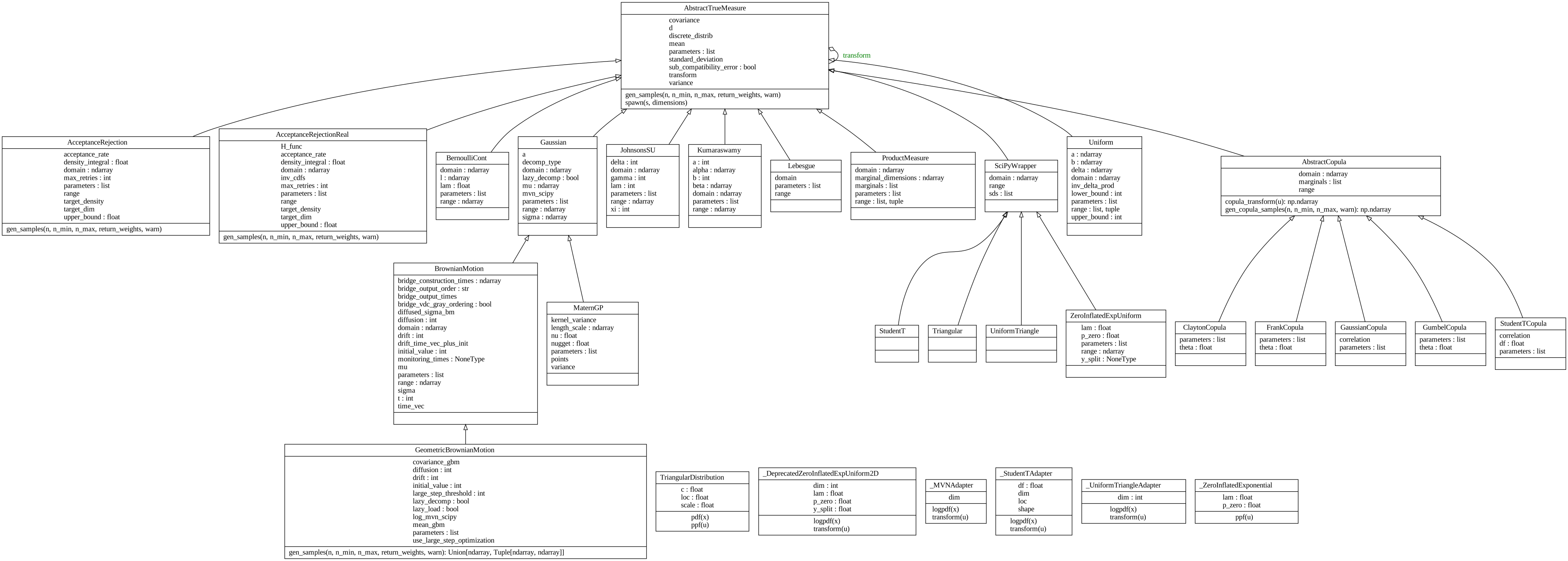
True Measures

UML Overview

AbstractTrueMeasure

Bases: object

Source code in qmcpy/true_measure/abstract_true_measure.py

def __init__(self):
    prefix = "A concrete implementation of TrueMeasure must have "
    if not hasattr(self, "domain"):
        raise ParameterError(
            prefix
            + "self.domain, 2xd ndarray of domain lower bounds (first col) and upper bounds (second col)"
        )
    if not hasattr(self, "range"):
        raise ParameterError(
            prefix
            + "self.range, 2xd ndarray of range lower bounds (first col) and upper bounds (second col)"
        )
    if not hasattr(self, "parameters"):
        self.parameters = []

__call__

__call__(n=None, n_min=None, n_max=None, return_weights=False, warn=True)

• If just n is supplied, generate samples from the sequence at indices 0,...,n-1.
• If n_min and n_max are supplied, generate samples from the sequence at indices n_min,...,n_max-1.
• If n and n_min are supplied, then generate samples from the sequence at indices n,...,n_min-1.

Parameters:

Name	Type	Description	Default
n	Union[None, int]	Number of points to generate.	None
n_min	Union[None, int]	Starting index of sequence.	None
n_max	Union[None, int]	Final index of sequence.	None
return_weights	bool	If True, return weights as well	False
warn	bool	If False, disable warnings when generating samples.	True

Returns:

Name	Type	Description
t	ndarray	Samples from the sequence. If replications is None then this will be of size (n_max-n_min) \(\times\) dimension If replications is a positive int, then t will be of size replications \(\times\) (n_max-n_min) \(\times\) dimension
weights	ndarray	Only returned when return_weights=True. The Jacobian weights for the transformation

Source code in qmcpy/true_measure/abstract_true_measure.py

def __call__(self, n=None, n_min=None, n_max=None, return_weights=False, warn=True):
    r"""
    - If just `n` is supplied, generate samples from the sequence at indices 0,...,`n`-1.
    - If `n_min` and `n_max` are supplied, generate samples from the sequence at indices `n_min`,...,`n_max`-1.
    - If `n` and `n_min` are supplied, then generate samples from the sequence at indices `n`,...,`n_min`-1.

    Args:
        n (Union[None, int]): Number of points to generate.
        n_min (Union[None, int]): Starting index of sequence.
        n_max (Union[None, int]): Final index of sequence.
        return_weights (bool): If `True`, return `weights` as well
        warn (bool): If `False`, disable warnings when generating samples.

    Returns:
        t (np.ndarray): Samples from the sequence.

            - If `replications` is `None` then this will be of size (`n_max`-`n_min`) $\times$ `dimension`
            - If `replications` is a positive int, then `t` will be of size `replications` $\times$ (`n_max`-`n_min`) $\times$ `dimension`
        weights (np.ndarray): Only returned when `return_weights=True`. The Jacobian weights for the transformation
    """
    return self.gen_samples(
        n=n, n_min=n_min, n_max=n_max, return_weights=return_weights, warn=warn
    )

spawn

spawn(s=1, dimensions=None)

Spawn new instances of the current true measure but with new seeds and dimensions. Used by multi-level QMC algorithms which require different seeds and dimensions on each level.

Note

Use replications instead of using spawn when possible, e.g., when spawning copies which all have the same dimension.

Parameters:

Name	Type	Description	Default
s	int	Number of copies to spawn	1
dimensions	ndarray	Length s array of dimensions for each copy. Defaults to the current dimension.	None

Returns:

Name	Type	Description
spawned_true_measures	list	True measure with new seeds and dimensions.

Source code in qmcpy/true_measure/abstract_true_measure.py

def spawn(self, s=1, dimensions=None):
    r"""
    Spawn new instances of the current true measure but with new seeds and dimensions.
    Used by multi-level QMC algorithms which require different seeds and dimensions on each level.

    Note:
        Use `replications` instead of using `spawn` when possible, e.g., when spawning copies which all have the same dimension.

    Args:
        s (int): Number of copies to spawn
        dimensions (np.ndarray): Length `s` array of dimensions for each copy. Defaults to the current dimension.

    Returns:
        spawned_true_measures (list): True measure with new seeds and dimensions.
    """
    sampler = self.discrete_distrib if self.transform == self else self.transform
    sampler_spawns = sampler.spawn(s=s, dimensions=dimensions)
    spawned_true_measures = [None] * len(sampler_spawns)
    for i in range(s):
        spawned_true_measures[i] = self._spawn(
            sampler_spawns[i], sampler_spawns[i].d
        )
    return spawned_true_measures

SciPyWrapper

Bases: AbstractTrueMeasure

True measure that wraps SciPy style distributions.

This class keeps the original behavior of SciPyWrapper with independent 1D marginals and adds an optional "joint" mode for dependent distributions.

Examples:

Independent marginals from scipy.stats:

>>> import scipy.stats as stats
>>> tm = SciPyWrapper(
...     sampler=DigitalNetB2(3, seed=7),
...     scipy_distribs=[
...         stats.uniform(loc=1, scale=2),
...         stats.norm(loc=0, scale=1),
...         stats.gamma(a=5, loc=0, scale=2)])
>>> x = tm(2)
>>> x.shape
(2, 3)

Joint multivariate normal passed as a single object:

>>> mvn = stats.multivariate_normal(
...     mean=[0.0, 0.0],
...     cov=[[1.0, 0.8], [0.8, 1.0]])
>>> tm_joint = SciPyWrapper(DigitalNetB2(2, seed=7), mvn)
>>> tm_joint(2).shape
(2, 2)

2D Student t distribution (independent marginals):

>>> df = 5
>>> true_measure = SciPyWrapper(
...     sampler=DigitalNetB2(2, seed=13),
...     scipy_distribs=[
...         stats.t(df=df, loc=0.0, scale=1.0),
...         stats.t(df=df, loc=1.0, scale=2.0),
...     ],
... )
>>> xs = true_measure(4)
>>> xs.shape
(4, 2)

Parameters

sampler : AbstractDiscreteDistribution Low discrepancy or iid sampler in dimension d, living on [0,1)^d. scipy_distribs : One of the following:

- A single SciPy 1D continuous frozen distribution.
- A list of such frozen distributions (independent marginals).
- A custom 1D distribution object with ``ppf`` and ``pdf`` or
  ``logpdf`` methods.
- A joint object with:
    * ``transform(u)`` method
    * optional ``logpdf(x)`` method
    * ``dim`` or ``dimension`` attribute (otherwise ``sampler.d``).

Source code in qmcpy/true_measure/scipy_wrapper.py

def __init__(self, sampler, scipy_distribs):
    """
    Parameters
    ----------
    sampler : AbstractDiscreteDistribution
        Low discrepancy or iid sampler in dimension d, living on [0,1)^d.
    scipy_distribs :
        One of the following:

        - A single SciPy 1D continuous frozen distribution.
        - A list of such frozen distributions (independent marginals).
        - A custom 1D distribution object with ``ppf`` and ``pdf`` or
          ``logpdf`` methods.
        - A joint object with:
            * ``transform(u)`` method
            * optional ``logpdf(x)`` method
            * ``dim`` or ``dimension`` attribute (otherwise ``sampler.d``).
    """
    self.domain = np.array([[0.0, 1.0]])

    if not isinstance(sampler, AbstractDiscreteDistribution):
        if not (
            hasattr(sampler, "d")
            and hasattr(sampler, "gen_samples")
            and callable(sampler.gen_samples)
        ):
            raise ParameterError(
                "SciPyWrapper requires sampler be an AbstractDiscreteDistribution."
            )
    self._parse_sampler(sampler)

    # Remember what the user originally passed in so that _spawn can reuse it.
    self._user_distrib_arg = scipy_distribs

    # Flags and holders for the two modes.
    self._is_joint = False
    self._joint = None
    self._joint_has_logpdf = False
    self._warned_missing_pdf = False

    if self._looks_like_joint(scipy_distribs):
        # Configure joint mode.
        self._setup_joint(scipy_distribs)
    else:
        # Configure independent marginals mode.
        self._setup_marginals(scipy_distribs)

    super(SciPyWrapper, self).__init__()

ProductMeasure

Bases: AbstractTrueMeasure

Product true measure for independent composition of marginal true measures.

ProductMeasure represents an independent product of smaller true measures. Each marginal may be one-dimensional or multidimensional. If the marginal true measures have dimensions

d_1, d_2, ..., d_k,

then the product measure has total dimension

d = d_1 + d_2 + ... + d_k.

A single d-dimensional outer sampler is used. Its unit-cube samples are split into coordinate blocks, one block for each marginal true measure. Each marginal transforms its own block, and the transformed blocks are concatenated back together.

For example, if the marginals are

marginal 1: 2D Gaussian
marginal 2: 1D zero-inflated exponential

then ProductMeasure uses a 3D sampler and returns samples with three coordinates. The first two coordinates come from the Gaussian marginal, and the third coordinate comes from the zero-inflated exponential marginal.

The marginal true measures still have their own samplers because QMCPy's current AbstractTrueMeasure API requires every true measure to be constructed with one. A DummySampler is useful for this construction placeholder role. Inside ProductMeasure, marginal samplers are not sampled directly when product samples are generated. The marginals provide dimension, range, transform, and weight behavior. A future samplerless/template true-measure mode may be useful, but that is separate from this class.

Notes

Exact product weights are supported for direct marginal true measures. For recursively composed marginal measures, sampling is supported through QMCPy's recursive transform helper, but exact final-space product weights are not currently implemented here.

Examples

Combine two one-dimensional uniform true measures:

from qmcpy import DigitalNetB2, DummySampler, ProductMeasure, Uniform marginals = [ ... Uniform(DummySampler(1), lower_bound=0, upper_bound=2), ... Uniform(DummySampler(1), lower_bound=10, upper_bound=12), ... ] pm = ProductMeasure(sampler=DigitalNetB2(2, seed=9), marginals=marginals) x = pm(4) x.shape (4, 2) bool(((0 <= x[:, 0]) & (x[:, 0] <= 2)).all()) True

The outer sampler controls replications:

pm = ProductMeasure( ... sampler=DigitalNetB2(2, seed=9, replications=3), ... marginals=marginals, ... ) pm(4).shape (3, 4, 2)

The DummySampler marginal samplers are only construction placeholders required by the current AbstractTrueMeasure interface. ProductMeasure samples from its own outer sampler.

Marginals may have different dimensions:

import numpy as np from qmcpy import Gaussian marginals = [ ... Gaussian( ... DummySampler(2), ... mean=[0, 0], ... covariance=np.eye(2), ... ), ... Uniform(DummySampler(1), lower_bound=10, upper_bound=12), ... ] pm = ProductMeasure(sampler=DigitalNetB2(3, seed=12), marginals=marginals) pm(4).shape (4, 3)

Initialize a product measure from one sampler and several marginals.

Parameters

sampler : AbstractDiscreteDistribution The sampler for the whole product measure. Its dimension must equal the sum of the marginal dimensions.

list or tuple of AbstractTrueMeasure

Independent true measures to place side by side. A marginal may itself be multidimensional.

Why one sampler?

The product measure should be driven by one total-dimensional QMC point set. We do not generate separate QMC samples from each marginal. Instead, one sample u in [0,1]^d is split into blocks:

u = (u_marginal_1, u_marginal_2, ..., u_marginal_k).

This preserves the intended total-dimensional QMC construction.

Source code in qmcpy/true_measure/product_measure.py

def __init__(self, sampler, marginals):
    """
    Initialize a product measure from one sampler and several marginals.

    Parameters
    ----------
    sampler : AbstractDiscreteDistribution
        The sampler for the whole product measure. Its dimension must
        equal the sum of the marginal dimensions.

    marginals : list or tuple of AbstractTrueMeasure
        Independent true measures to place side by side. A marginal may
        itself be multidimensional.

    Why one sampler?
    ----------------
    The product measure should be driven by one total-dimensional QMC
    point set. We do not generate separate QMC samples from each marginal.
    Instead, one sample u in [0,1]^d is split into blocks:

        u = (u_marginal_1, u_marginal_2, ..., u_marginal_k).

    This preserves the intended total-dimensional QMC construction.
    """
    if not isinstance(marginals, (list, tuple)) or len(marginals) == 0:
        raise ParameterError("ProductMeasure requires a nonempty list of marginals.")

    if not all(isinstance(marginal, AbstractTrueMeasure) for marginal in marginals):
        raise ParameterError(
            "Each ProductMeasure marginal must be an AbstractTrueMeasure instance."
        )

    if not isinstance(sampler, AbstractDiscreteDistribution):
        raise ParameterError(
            "ProductMeasure sampler must be an AbstractDiscreteDistribution."
        )

    self.parameters = ["marginals"]
    # ProductMeasure uses only the sampler passed directly to ProductMeasure
    # to generate product samples.
    #
    # Marginal true measures also contain samplers because QMCPy's current
    # AbstractTrueMeasure interface requires true measures to be constructed
    # with an attached discrete distribution. Inside ProductMeasure, those
    # marginal samplers are not sampled. The marginals are used for their
    # dimension, range, transform, and weight behavior.
    self.marginals = list(marginals)
    for marginal in self.marginals:
        target_dim = getattr(marginal, "target_dim", marginal.d)
        if target_dim != marginal.d:
            raise DimensionError(
                "ProductMeasure marginals must be dimension-preserving "
                "block transforms. Marginal target dimension "
                f"{target_dim} does not match sampler dimension {marginal.d}."
            )

    self.marginal_dimensions = np.array(
        [marginal.d for marginal in self.marginals], dtype=int
    )
    self._split_indices = np.cumsum(self.marginal_dimensions)[:-1]

    self._total_marginal_dimension = int(self.marginal_dimensions.sum())
    if sampler.d != self._total_marginal_dimension:
        raise DimensionError(
            "ProductMeasure sampler dimension must equal the sum of marginal "
            f"dimensions ({sampler.d} != {self._total_marginal_dimension})."
        )

    self.domain = np.array([[0.0, 1.0]])
    self._parse_sampler(sampler)

    self.range = np.vstack(
        [
            self._expand_bounds(marginal.range, marginal.d, "range")
            for marginal in self.marginals
        ]
    )

    super(ProductMeasure, self).__init__()

StudentT

Bases: SciPyWrapper

Convenience true measure: multivariate Student t.

Source code in qmcpy/true_measure/student_t.py

def __init__(self, sampler, loc, shape, df):
    super().__init__(
        sampler=sampler,
        scipy_distribs=_StudentTAdapter(loc=loc, shape=shape, df=df),
    )

Triangular

Bases: SciPyWrapper

Convenience TrueMeasure wrapper around TriangularDistribution.

Source code in qmcpy/true_measure/triangular.py

def __init__(self, sampler, c=0.5, loc=0.0, scale=1.0):
    super().__init__(
        sampler=sampler,
        scipy_distribs=TriangularDistribution(c=c, loc=loc, scale=scale),
    )

UniformTriangle

Bases: SciPyWrapper

Uniform distribution on the triangle {(x, y): 0 <= y <= x <= 1}.

Example:

tm = UniformTriangle(sampler=DigitalNetB2(2, seed=7)) x = tm(4) x.shape (4, 2) bool(np.all(x[:, 1] <= x[:, 0])) True

Source code in qmcpy/true_measure/uniform_triangle.py

def __init__(self, sampler):
    super().__init__(sampler=sampler, scipy_distribs=_UniformTriangleAdapter())

ZeroInflatedExpUniform

Bases: SciPyWrapper

One-dimensional zero-inflated exponential true measure.

The y_split keyword is retained temporarily for backward compatibility with the deprecated two-dimensional construction.

Examples

Without replications:

from qmcpy import DigitalNetB2, ZeroInflatedExpUniform tm = ZeroInflatedExpUniform( ... DigitalNetB2(1, seed=7), p_zero=0.4, lam=1.5 ... ) x = tm(8) x array([[0. ], [0.76621559], [0. ], [0.18405583], [0.08112272], [1.19997153], [0. ], [0.33259467]]) x.shape (8, 1) bool((x >= 0).all()) True tm ZeroInflatedExpUniform (AbstractTrueMeasure) p_zero 0.400 lam 1.500 mean 0.400 variance 0.373 standard_deviation 0.611

Covariance is omitted because the measure is one dimensional (a 1x1 covariance would simply repeat the variance):

tm.mean 0.39999999999999997 tm.variance 0.3733333333333333 tm.standard_deviation 0.6110100926607787

With independent replications:

tm = ZeroInflatedExpUniform( ... DigitalNetB2(1, seed=7, replications=2), ... p_zero=0.4, ... lam=1.5, ... ) x = tm(8) x array([[[0.51197024], [0. ], [2.54258665], [0.03368876], [0.2192598 ], [0. ], [0.85384192], [0. ]], [[1.3024994 ], [0.03378461], [0.20489897], [0. ], [0.58638285], [0. ], [0.35227285], [0. ]]]) x.shape (2, 8, 1) bool((x >= 0).all()) True

Source code in qmcpy/true_measure/zero_inflated_exp_uniform.py

def __init__(self, sampler, p_zero=0.4, lam=1.5, y_split=None):
    if y_split is not None:
        warnings.warn(
            "`y_split` is deprecated. The 2D zero-inflated "
            "exponential-uniform construction is retained only for "
            "backward compatibility. Prefer the 1D "
            "ZeroInflatedExpUniform interface.",
            DeprecationWarning,
            stacklevel=2,
        )

        if sampler.d == 2:
            scipy_distribs = _DeprecatedZeroInflatedExpUniform2D(
                p_zero=p_zero,
                lam=lam,
                y_split=y_split,
            )
            self._deprecated_2d_y_split = True
        elif sampler.d == 1:
            scipy_distribs = _ZeroInflatedExponential(
                p_zero=p_zero,
                lam=lam,
            )
            self._deprecated_2d_y_split = False
        else:
            raise DimensionError(
                "ZeroInflatedExpUniform with deprecated y_split requires "
                "a one- or two-dimensional sampler."
            )
    else:
        if sampler.d != 1:
            raise DimensionError(
                "ZeroInflatedExpUniform requires a one-dimensional sampler."
            )

        scipy_distribs = _ZeroInflatedExponential(
            p_zero=p_zero,
            lam=lam,
        )
        self._deprecated_2d_y_split = False

    super().__init__(
        sampler=sampler,
        scipy_distribs=scipy_distribs,
    )

    self.parameters = ["p_zero", "lam"]
    self.p_zero = float(p_zero)
    self.lam = float(lam)
    self.y_split = y_split
    if self._deprecated_2d_y_split:
        self.parameters.append("y_split")
        self.range = np.array([[0.0, np.inf], [0.0, 1.0]])
    else:
        # Moments are only defined for the (non-deprecated) 1D
        # zero-inflated exponential. Covariance is intentionally omitted:
        # for a one-dimensional measure it would be a 1x1 matrix whose only
        # entry equals the variance.
        mean, variance = self._compute_moments()
        self._mean = self._read_only_array(mean)
        self._variance = self._read_only_array(variance)
        self._standard_deviation = self._read_only_array(np.sqrt(variance))
        self.parameters += [
            "mean",
            "variance",
            "standard_deviation",
        ]

AbstractCopula

Bases: AbstractTrueMeasure

Abstract base class for copula TrueMeasures.

A copula layer maps independent uniform input points to dependent uniform points on the unit cube:

\[ U \in [0,1]^d \mapsto V = T(U) \in [0,1]^d. \]

The base class then applies marginal quantile functions to obtain final target samples,

\[ X_j = F_j^{-1}(V_j). \]

SciPy calls the quantile function ppf. Concrete subclasses implement _transform_to_uniform for the family-specific copula sampling transform.

Source code in qmcpy/true_measure/copula.py

def __init__(self, sampler, marginals):
    self.domain = np.array([[0, 1]])
    self._parse_sampler(sampler)

    self.marginals = _validate_marginals(marginals)
    _validate_dimension(self, self.marginals)
    self.range = _build_marginal_range(self.marginals)
    self._warned_missing_weight = False

    super(AbstractCopula, self).__init__()

copula_transform

copula_transform(u)

Apply only the copula layer U -> V.

Parameters:

Name	Type	Description	Default
u	ndarray	Independent uniform points on [0,1]^d.	required

Returns:

Type	Description
ndarray	np.ndarray: Dependent uniform points on [0,1]^d.

Source code in qmcpy/true_measure/copula.py

def copula_transform(self, u) -> np.ndarray:
    r"""
    Apply only the copula layer ``U -> V``.

    Args:
        u (np.ndarray): Independent uniform points on ``[0,1]^d``.

    Returns:
        np.ndarray: Dependent uniform points on ``[0,1]^d``.
    """
    return self._transform_to_uniform(u)

gen_copula_samples

gen_copula_samples(n=None, n_min=None, n_max=None, warn=True)

Generate dependent copula uniforms without applying marginal quantiles.

This is the copula-only workflow U -> V. Calling the object itself keeps the ordinary TrueMeasure workflow U -> V -> X.

Source code in qmcpy/true_measure/copula.py

def gen_copula_samples(
    self, n=None, n_min=None, n_max=None, warn=True
) -> np.ndarray:
    r"""
    Generate dependent copula uniforms without applying marginal quantiles.

    This is the copula-only workflow ``U -> V``. Calling the object itself
    keeps the ordinary TrueMeasure workflow ``U -> V -> X``.
    """
    u = self.discrete_distrib(n=n, n_min=n_min, n_max=n_max, warn=warn)
    if self.transform != self:
        u = self.transform._jacobian_transform_r(x=u, return_weights=False)
    return self._transform_to_uniform(u)

GaussianCopula

Bases: AbstractCopula

Gaussian copula transform with user supplied univariate marginals.

This TrueMeasure separates the dependence model from the marginal distributions:

1. map independent uniforms through scipy.stats.norm.ppf;
2. inject Gaussian dependence with a Cholesky factor of the correlation;
3. map back to dependent uniforms with scipy.stats.norm.cdf;
4. apply each marginal quantile function.

SciPy calls the quantile function ppf. The marginal objects must expose this method. If they also expose cdf and pdf or logpdf, then _weight computes the Gaussian copula joint density. Otherwise weights are treated as one with a warning.

Examples:

>>> import numpy as np
>>> import scipy.stats as stats
>>> sampler = DigitalNetB2(2, seed=7)
>>> marginals = [stats.beta(a=2, b=5), stats.gamma(a=3, scale=2)]
>>> corr = [[1.0, 0.6], [0.6, 1.0]]
>>> tm = GaussianCopula(sampler, marginals=marginals, correlation=corr)
>>> x = tm(4)
>>> x.shape
(4, 2)
>>> bool(np.isfinite(x).all())
True
>>> tm
GaussianCopula (AbstractTrueMeasure)
    marginals       [<...rv_continuous_frozen object at ...>
                     <...rv_continuous_frozen object at ...>]
    correlation     [[1.  0.6]
                     [0.6 1. ]]
>>> rep_marginals = [stats.beta(a=2, b=5), stats.gamma(a=3, scale=2), stats.expon()]
>>> rep_corr = [[1.0, 0.6, 0.3],
...             [0.6, 1.0, 0.2],
...             [0.3, 0.2, 1.0]]
>>> rep_tm = GaussianCopula(
...     DigitalNetB2(3, seed=7, replications=2),
...     marginals=rep_marginals,
...     correlation=rep_corr,
... )
>>> samples = rep_tm(4)
>>> samples.shape
(2, 4, 3)
>>> bool(np.isfinite(samples).all())
True
>>> GaussianCopula(DigitalNetB2(1, seed=7), marginals=[stats.norm()], correlation=[[1.0]])(4).shape
(4, 1)

References:

1. Roger B. Nelsen. An Introduction to Copulas. Second Edition, Springer Series in Statistics, Springer, 2006. doi:10.1007/0-387-28678-0.

2. Mathieu Cambou, Marius Hofert, and Christiane Lemieux. "Quasi-random numbers for copula models." arXiv:1508.03483.

Parameters:

Name	Type	Description	Default
sampler	Union[AbstractDiscreteDistribution, AbstractTrueMeasure]	A sampler or transform whose range is the unit cube.	required
marginals	list	Length d list of SciPy-like univariate distributions implementing a quantile function, called ppf in SciPy.	required
correlation	ndarray	d x d positive definite correlation matrix.	required

Source code in qmcpy/true_measure/gaussian_copula.py

def __init__(self, sampler, marginals, correlation):
    r"""
    Args:
        sampler (Union[AbstractDiscreteDistribution, AbstractTrueMeasure]):
            A sampler or transform whose range is the unit cube.
        marginals (list): Length d list of SciPy-like univariate
            distributions implementing a quantile function, called ``ppf``
            in SciPy.
        correlation (np.ndarray): d x d positive definite correlation matrix.
    """
    self.parameters = ["marginals", "correlation"]
    super(GaussianCopula, self).__init__(sampler=sampler, marginals=marginals)
    self.correlation = _validate_correlation_matrix(correlation, self.d)

    self._gaussian_transform = Gaussian(
        sampler,
        mean=np.zeros(self.d),
        covariance=self.correlation,
        decomp_type="Cholesky",
    )
    # Gaussian copula density:
    # c(u) = |R|^{-1/2} exp(-0.5 z^T (R^{-1} - I) z), z = Phi^{-1}(u).
    # The identity subtraction removes the independent standard-normal density
    # already accounted for by the marginal normal transforms.
    self._corr_inv_minus_eye = np.linalg.inv(self.correlation) - np.eye(self.d)
    _, self._logdet_corr = np.linalg.slogdet(self.correlation)

StudentTCopula

Bases: AbstractCopula

Student-t copula transform with user supplied univariate marginals.

This TrueMeasure uses the same marginal workflow as GaussianCopula, but builds dependent uniforms through a multivariate Student-t copula with correlation matrix correlation and degrees of freedom df.

The transform uses the inverse Rosenblatt construction for the multivariate Student-t distribution. This is equivalent in distribution to the standard correlated-normal plus shared chi-square scaling construction, but it only needs d deterministic uniforms from the base QMCPy sampler. It is not the incorrect shortcut of applying univariate t.ppf, a Cholesky factor, and then univariate t.cdf.

Examples:

>>> import numpy as np
>>> import scipy.stats as stats
>>> sampler = DigitalNetB2(2, seed=7)
>>> marginals = [stats.norm(), stats.gamma(a=3, scale=2)]
>>> corr = [[1.0, 0.6], [0.6, 1.0]]
>>> tm = StudentTCopula(sampler, marginals=marginals, correlation=corr, df=4)
>>> x = tm(4)
>>> x.shape
(4, 2)
>>> bool(np.isfinite(x).all())
True
>>> tm
StudentTCopula (AbstractTrueMeasure)
    marginals       [<...rv_continuous_frozen object at ...>
                     <...rv_continuous_frozen object at ...>]
    correlation     [[1.  0.6]
                     [0.6 1. ]]
    df              2^(2)
>>> rep_marginals = [stats.norm(), stats.gamma(a=3, scale=2), stats.expon()]
>>> rep_corr = [[1.0, 0.6, 0.3],
...             [0.6, 1.0, 0.2],
...             [0.3, 0.2, 1.0]]
>>> rep_tm = StudentTCopula(
...     DigitalNetB2(3, seed=7, replications=2),
...     marginals=rep_marginals,
...     correlation=rep_corr,
...     df=4,
... )
>>> samples = rep_tm(4)
>>> samples.shape
(2, 4, 3)
>>> bool(np.isfinite(samples).all())
True
>>> StudentTCopula(DigitalNetB2(1, seed=7), marginals=[stats.norm()], correlation=[[1.0]], df=4)(4).shape
(4, 1)
>>> StudentTCopula(DigitalNetB2(2, seed=7), marginals=marginals, correlation=corr, df=1)(4).shape
(4, 2)

References:

1. Roger B. Nelsen. An Introduction to Copulas. Second Edition, Springer Series in Statistics, Springer, 2006. doi:10.1007/0-387-28678-0.

2. Mathieu Cambou, Marius Hofert, and Christiane Lemieux. "Quasi-random numbers for copula models." arXiv:1508.03483.

3. M. Rosenblatt. "Remarks on a Multivariate Transformation." The Annals of Mathematical Statistics 23(3), 470-472, 1952. doi:10.1214/aoms/1177729394.

Parameters:

Name	Type	Description	Default
sampler	Union[AbstractDiscreteDistribution, AbstractTrueMeasure]	A sampler or transform whose range is the unit cube.	required
marginals	list	Length d list of SciPy-like univariate distributions implementing a quantile function, called ppf in SciPy.	required
correlation	ndarray	d x d positive definite correlation matrix.	required
df	float	Positive Student-t degrees of freedom.	required

Source code in qmcpy/true_measure/student_t_copula.py

def __init__(self, sampler, marginals, correlation, df):
    r"""
    Args:
        sampler (Union[AbstractDiscreteDistribution, AbstractTrueMeasure]):
            A sampler or transform whose range is the unit cube.
        marginals (list): Length d list of SciPy-like univariate
            distributions implementing a quantile function, called ``ppf``
            in SciPy.
        correlation (np.ndarray): d x d positive definite correlation matrix.
        df (float): Positive Student-t degrees of freedom.
    """
    self.parameters = ["marginals", "correlation", "df"]
    super(StudentTCopula, self).__init__(sampler=sampler, marginals=marginals)
    self.correlation = _validate_correlation_matrix(correlation, self.d)
    self.df = self._parse_df(df)

    self._mvt_scipy = None
    if hasattr(stats, "multivariate_t"):
        self._mvt_scipy = stats.multivariate_t(
            loc=np.zeros(self.d), shape=self.correlation, df=self.df
        )

ClaytonCopula

Bases: AbstractCopula

Clayton copula transform with user supplied marginals.

This implementation supports general dimension for theta > 0. It maps independent uniforms to Clayton-dependent uniforms using the conditional inverse / inverse Rosenblatt transform. For coordinate j after observing the previous m = j - 1 coordinates, the conditional inverse is

\[ v = \left(1 + A \left(w^{-\theta/(1 + m \theta)} - 1\right)\right)^{-1/\theta}, \]

where A = 1 + sum(phi(u_i)) over previous coordinates and phi(u) = u^{-theta} - 1.

The base AbstractCopula class then applies each marginal quantile function. SciPy calls the quantile function ppf.

Clayton copulas have positive lower-tail dependence for theta > 0.

Examples:

>>> import numpy as np
>>> import scipy.stats as stats
>>> sampler = DigitalNetB2(2, seed=7)
>>> marginals = [stats.expon(), stats.gamma(a=3)]
>>> tm = ClaytonCopula(sampler, marginals=marginals, theta=2.0)
>>> x = tm(4)
>>> x.shape
(4, 2)
>>> bool(np.isfinite(x).all())
True
>>> tm
ClaytonCopula (AbstractTrueMeasure)
    marginals       [<...rv_continuous_frozen object at ...>
                     <...rv_continuous_frozen object at ...>]
    theta           2^(1)
>>> rep_marginals = [stats.expon(), stats.gamma(a=3), stats.beta(a=2, b=5)]
>>> rep_tm = ClaytonCopula(
...     DigitalNetB2(3, seed=7, replications=2),
...     marginals=rep_marginals,
...     theta=2.0,
... )
>>> samples = rep_tm(4)
>>> samples.shape
(2, 4, 3)
>>> bool(np.isfinite(samples).all())
True
>>> ClaytonCopula(DigitalNetB2(3, seed=7), marginals=[stats.uniform()] * 3, theta=2.0)(4).shape
(4, 3)
>>> ClaytonCopula(DigitalNetB2(2, seed=7), marginals=marginals, theta=1e-8)(4).shape
(4, 2)

References:

1. Roger B. Nelsen. An Introduction to Copulas. Second Edition, Springer Series in Statistics, Springer, 2006. doi:10.1007/0-387-28678-0.

2. Mathieu Cambou, Marius Hofert, and Christiane Lemieux. "Quasi-random numbers for copula models." arXiv:1508.03483.

3. Marius Hofert, Martin Maechler, and Alexander J. McNeil. "Likelihood inference for Archimedean copulas in high dimensions under known margins." Journal of Multivariate Analysis 110, 133-150, 2012. doi:10.1016/j.jmva.2012.02.019.

Parameters:

Name	Type	Description	Default
sampler	Union[AbstractDiscreteDistribution, AbstractTrueMeasure]	A sampler or transform whose range is the unit cube.	required
marginals	list	Length d list of SciPy-like univariate distributions implementing a quantile function, called ppf in SciPy.	required
theta	float	Positive Clayton dependence parameter.	required

Source code in qmcpy/true_measure/clayton_copula.py

def __init__(self, sampler, marginals, theta):
    r"""
    Args:
        sampler (Union[AbstractDiscreteDistribution, AbstractTrueMeasure]):
            A sampler or transform whose range is the unit cube.
        marginals (list): Length d list of SciPy-like univariate
            distributions implementing a quantile function, called ``ppf``
            in SciPy.
        theta (float): Positive Clayton dependence parameter.
    """
    self.parameters = ["marginals", "theta"]
    super(ClaytonCopula, self).__init__(sampler=sampler, marginals=marginals)
    self.theta = self._parse_theta(theta)

GumbelCopula

Bases: AbstractCopula

Gumbel copula transform with user supplied marginals.

This implementation supports general dimension for theta >= 1. It maps independent uniforms to Gumbel-dependent uniforms by numerically inverting the conditional CDFs from the inverse Rosenblatt construction. The base AbstractCopula class then applies marginal quantile functions. SciPy calls the quantile function ppf.

Gumbel copulas have positive upper-tail dependence for theta > 1. The boundary case theta = 1 is the independent copula.

Examples:

>>> import numpy as np
>>> import scipy.stats as stats
>>> sampler = DigitalNetB2(2, seed=7)
>>> marginals = [stats.expon(), stats.gamma(a=3)]
>>> tm = GumbelCopula(sampler, marginals=marginals, theta=2.0)
>>> x = tm(4)
>>> x.shape
(4, 2)
>>> bool(np.isfinite(x).all())
True
>>> tm
GumbelCopula (AbstractTrueMeasure)
    marginals       [<...rv_continuous_frozen object at ...>
                     <...rv_continuous_frozen object at ...>]
    theta           2^(1)
>>> rep_marginals = [stats.expon(), stats.gamma(a=3), stats.beta(a=2, b=5)]
>>> rep_tm = GumbelCopula(
...     DigitalNetB2(3, seed=7, replications=2),
...     marginals=rep_marginals,
...     theta=2.0,
... )
>>> samples = rep_tm(4)
>>> samples.shape
(2, 4, 3)
>>> bool(np.isfinite(samples).all())
True
>>> GumbelCopula(DigitalNetB2(3, seed=7), marginals=[stats.uniform()] * 3, theta=2.0)(4).shape
(4, 3)
>>> independent_tm = GumbelCopula(DigitalNetB2(2, seed=7), marginals=[stats.uniform(), stats.uniform()], theta=1.0)
>>> independent_samples = independent_tm(4)
>>> independent_samples.shape
(4, 2)
>>> bool(((0 <= independent_samples) & (independent_samples <= 1)).all())
True

References:

1. Roger B. Nelsen. An Introduction to Copulas. Second Edition, Springer Series in Statistics, Springer, 2006. doi:10.1007/0-387-28678-0.

2. Mathieu Cambou, Marius Hofert, and Christiane Lemieux. "Quasi-random numbers for copula models." arXiv:1508.03483.

3. Marius Hofert, Martin Maechler, and Alexander J. McNeil. "Likelihood inference for Archimedean copulas in high dimensions under known margins." Journal of Multivariate Analysis 110, 133-150, 2012. doi:10.1016/j.jmva.2012.02.019.

Parameters:

Name	Type	Description	Default
sampler	Union[AbstractDiscreteDistribution, AbstractTrueMeasure]	A sampler or transform whose range is the unit cube.	required
marginals	list	Length d list of SciPy-like univariate distributions implementing a quantile function, called ppf in SciPy.	required
theta	float	Gumbel dependence parameter, requiring theta >= 1.	required

Source code in qmcpy/true_measure/gumbel_copula.py

def __init__(self, sampler, marginals, theta):
    r"""
    Args:
        sampler (Union[AbstractDiscreteDistribution, AbstractTrueMeasure]):
            A sampler or transform whose range is the unit cube.
        marginals (list): Length d list of SciPy-like univariate
            distributions implementing a quantile function, called ``ppf``
            in SciPy.
        theta (float): Gumbel dependence parameter, requiring ``theta >= 1``.
    """
    self.parameters = ["marginals", "theta"]
    super(GumbelCopula, self).__init__(sampler=sampler, marginals=marginals)
    self.theta = self._parse_theta(theta)
    self._alpha = 1.0 / self.theta
    self._derivative_terms_cache = {}

FrankCopula

Bases: AbstractCopula

Frank copula transform with user supplied univariate marginals.

This implementation supports general dimension for theta > 0. Negative theta is supported only for the bivariate case, where the negative parameter Frank copula is valid. For dimensions greater than 2, theta must be positive.

The transform uses the inverse Rosenblatt construction for the Frank Archimedean copula. It maps independent uniforms to dependent uniforms by recursively inverting conditional CDFs. The base AbstractCopula class then applies each marginal quantile function. SciPy calls the quantile function ppf.

Examples:

>>> import numpy as np
>>> import scipy.stats as stats
>>> sampler = DigitalNetB2(3, seed=7)
>>> marginals = [stats.norm(), stats.gamma(a=3), stats.expon()]
>>> tm = FrankCopula(sampler, marginals=marginals, theta=5.0)
>>> x = tm(4)
>>> x.shape
(4, 3)
>>> bool(np.isfinite(x).all())
True
>>> tm
FrankCopula (AbstractTrueMeasure)
    marginals       [<...rv_continuous_frozen object at ...>
                     <...rv_continuous_frozen object at ...>
                     <...rv_continuous_frozen object at ...>]
    theta           5
>>> rep_tm = FrankCopula(
...     DigitalNetB2(3, seed=7, replications=2),
...     marginals=marginals,
...     theta=5.0,
... )
>>> samples = rep_tm(4)
>>> samples.shape
(2, 4, 3)
>>> bool(np.isfinite(samples).all())
True
>>> neg_tm = FrankCopula(DigitalNetB2(2, seed=7), marginals=[stats.uniform(), stats.uniform()], theta=-2.0)
>>> neg_samples = neg_tm(4)
>>> neg_samples.shape
(4, 2)
>>> bool(((0 <= neg_samples) & (neg_samples <= 1)).all())
True
>>> try:
...     FrankCopula(DigitalNetB2(3, seed=7), marginals=[stats.uniform()] * 3, theta=-2.0)
... except ParameterError as exc:
...     print(str(exc))
theta < 0 is only supported for d=2 FrankCopula.
>>> FrankCopula(DigitalNetB2(5, seed=7), marginals=[stats.uniform()] * 5, theta=5.0)(4).shape
(4, 5)

References:

1. Roger B. Nelsen. An Introduction to Copulas. Second Edition, Springer Series in Statistics, Springer, 2006. doi:10.1007/0-387-28678-0.

2. Mathieu Cambou, Marius Hofert, and Christiane Lemieux. "Quasi-random numbers for copula models." arXiv:1508.03483.

3. Marius Hofert, Martin Maechler, and Alexander J. McNeil. "Likelihood inference for Archimedean copulas in high dimensions under known margins." Journal of Multivariate Analysis 110, 133-150, 2012. doi:10.1016/j.jmva.2012.02.019.

Parameters:

Name	Type	Description	Default
sampler	Union[AbstractDiscreteDistribution, AbstractTrueMeasure]	A sampler or transform whose range is the unit cube.	required
marginals	list	Length d list of SciPy-like univariate distributions implementing a quantile function, called ppf in SciPy.	required
theta	float	Frank dependence parameter. Must be nonzero. Negative values are currently supported only for d=2.	required

Source code in qmcpy/true_measure/frank_copula.py

def __init__(self, sampler, marginals, theta):
    r"""
    Args:
        sampler (Union[AbstractDiscreteDistribution, AbstractTrueMeasure]):
            A sampler or transform whose range is the unit cube.
        marginals (list): Length d list of SciPy-like univariate
            distributions implementing a quantile function, called ``ppf``
            in SciPy.
        theta (float): Frank dependence parameter. Must be nonzero. Negative
            values are currently supported only for ``d=2``.
    """
    self.parameters = ["marginals", "theta"]
    super(FrankCopula, self).__init__(sampler=sampler, marginals=marginals)
    self.theta = self._parse_theta(theta)

    self._expm1_neg_theta = np.expm1(-self.theta)
    if self._expm1_neg_theta == 0 or not np.isfinite(self._expm1_neg_theta):
        raise ParameterError("theta is too close to 0 or too large in magnitude.")
    self._alpha = -self._expm1_neg_theta
    self._eulerian_cache = {}

Uniform

Bases: AbstractTrueMeasure

Uniform distribution, see https://en.wikipedia.org/wiki/Continuous_uniform_distribution.

Examples:

>>> true_measure = Uniform(DigitalNetB2(2,seed=7),lower_bound=[0,.5],upper_bound=[2,3])
>>> true_measure(4)
array([[1.44324713, 2.7873875 ],
       [0.32691107, 1.5741214 ],
       [1.97352511, 0.58590959],
       [0.8591331 , 1.89690854]])

The covariance is diagonal, so it is stored and shown in sparse form.

>>> true_measure
Uniform (AbstractTrueMeasure)
    lower_bound     [0.  0.5]
    upper_bound     [2 3]
    mean            [1.   1.75]
    variance        [0.333 0.521]
    standard_deviation [0.577 0.722]
    covariance      <DIAgonal sparse matrix of dtype 'float64'
        with 2 stored elements (1 diagonals) and shape (2, 2)>
        Coords Values
        (0, 0) 0.3333333333333333
        (1, 1) 0.5208333333333334

With independent replications

>>> x = Uniform(DigitalNetB2(3,seed=7,replications=2),lower_bound=[.25,.5,.75],upper_bound=[1.75,1.5,1.25])(4)
>>> x.shape
(2, 4, 3)
>>> x
array([[[0.61979915, 0.6821862 , 1.12366296],
        [1.27229355, 1.16169442, 0.9644598 ],
        [0.97209782, 1.29818233, 0.79100643],
        [1.62311988, 0.79520621, 1.13747905]],

       [[0.92315337, 1.35899604, 1.0027484 ],
        [1.05453886, 0.54353443, 0.91782473],
        [0.59821215, 0.79281506, 0.78420518],
        [1.37943573, 1.10241448, 1.13481488]]])

Parameters:

Name	Type	Description	Default
sampler	Union[AbstractDiscreteDistribution, AbstractTrueMeasure]	Either a discrete distribution from which to transform samples, or a true measure by which to compose a transform.	required
lower_bound	Union[float, ndarray]	Lower bound.	0
upper_bound	Union[float, ndarray]	Upper bound.	1

Source code in qmcpy/true_measure/uniform.py

def __init__(self, sampler, lower_bound=0, upper_bound=1):
    r"""
    Args:
        sampler (Union[AbstractDiscreteDistribution, AbstractTrueMeasure]): Either

            - a discrete distribution from which to transform samples, or
            - a true measure by which to compose a transform.
        lower_bound (Union[float, np.ndarray]): Lower bound.
        upper_bound (Union[float, np.ndarray]): Upper bound.
    """
    self.parameters = ["lower_bound", "upper_bound", "mean", "variance", "standard_deviation", "covariance"]
    self.domain = np.array([[0, 1]])
    self._parse_sampler(sampler)
    self.lower_bound = lower_bound
    self.upper_bound = upper_bound
    if np.isscalar(self.lower_bound):
        lower_bound = np.tile(self.lower_bound, self.d)
    if np.isscalar(self.upper_bound):
        upper_bound = np.tile(self.upper_bound, self.d)
    self.a = np.array(lower_bound, dtype=np.float64)
    self.b = np.array(upper_bound, dtype=np.float64)
    if len(self.a) != self.d or len(self.b) != self.d:
        raise DimensionError(
            "upper bound and lower bound must be of length dimension"
        )
    if not (np.all(np.isfinite(self.a)) and np.all(np.isfinite(self.b))):
        raise ParameterError("upper bound and lower bound must be finite")
    self.delta = self.b - self.a
    if np.any(self.delta <= 0):
        raise ParameterError(
            "upper bound must be strictly greater than lower bound"
        )
    mean = (self.a + self.b) / 2
    variance = self.delta**2 / 12
    self._set_moments(
        mean=mean,
        variance=variance,
        standard_deviation=self.delta / np.sqrt(12),
        covariance=diags(variance, format="dia"),
    )
    self.inv_delta_prod = 1 / self.delta.prod()
    self.range = np.hstack(
        (self.a.reshape((self.d, 1)), self.b.reshape((self.d, 1)))
    )
    super(Uniform, self).__init__()
    assert self.a.shape == (self.d,) and self.b.shape == (self.d,)

Gaussian

Bases: AbstractTrueMeasure

Gaussian (Normal) distribution as described in https://en.wikipedia.org/wiki/Multivariate_normal_distribution.

Note

• Normal is an alias for Gaussian

Examples:

>>> true_measure = Gaussian(DigitalNetB2(2,seed=7),mean=[1,2],covariance=[[9,4],[4,5]])
>>> true_measure(4)
array([[ 3.83994612,  1.19097885],
       [-1.9727727 ,  0.49405353],
       [ 5.87242307,  8.41341485],
       [ 0.61222205,  1.48402653]])
>>> true_measure
Gaussian (AbstractTrueMeasure)
    mean            [1. 2.]
    variance        [9. 5.]
    standard_deviation [3.    2.236]
    covariance      [[9. 4.]
                     [4. 5.]]
    decomp_type     PCA

With independent replications

>>> x = Gaussian(DigitalNetB2(3,seed=7,replications=2),mean=0,covariance=3)(4)
>>> x.shape
(2, 4, 3)
>>> x
array([[[-1.18721904, -1.57108272,  1.15371635],
        [ 0.81749123,  0.72242445, -0.31025434],
        [-0.0807895 ,  1.44651585, -2.41042379],
        [ 2.38133494, -0.93225637,  1.30817519]],

       [[-0.22304017,  1.86337427,  0.02386568],
        [ 0.15807672, -2.96365385, -0.73502346],
        [-1.26753687, -0.94427848, -2.57683314],
        [ 1.1844196 ,  0.44964332,  1.27760936]]])

Parameters:

Name	Type	Description	Default
sampler	Union[AbstractDiscreteDistribution, AbstractTrueMeasure]	Either a discrete distribution from which to transform samples, or a true measure by which to compose a transform.	required
mean	Union[float, ndarray]	Mean vector.	0.0
covariance	Union[float, ndarray]	Covariance matrix. A float or vector will be expanded into a diagonal matrix.	1.0
decomp_type	str	Method for decomposition for covariance matrix. Options include 'PCA' for principal component analysis, or 'Cholesky' for cholesky decomposition.	'PCA'

Source code in qmcpy/true_measure/gaussian.py

def __init__(self, sampler, mean=0.0, covariance=1.0, decomp_type="PCA"):
    """
    Args:
        sampler (Union[AbstractDiscreteDistribution, AbstractTrueMeasure]): Either

            - a discrete distribution from which to transform samples, or
            - a true measure by which to compose a transform.
        mean (Union[float, np.ndarray]): Mean vector.
        covariance (Union[float, np.ndarray]): Covariance matrix. A float or vector will be expanded into a diagonal matrix.
        decomp_type (str): Method for decomposition for covariance matrix. Options include

            - `'PCA'` for principal component analysis, or
            - `'Cholesky'` for cholesky decomposition.
    """
    self.parameters = ["mean", "variance", "standard_deviation", "covariance", "decomp_type"]
    # default to transform from standard uniform
    self.domain = np.array([[0, 1]])
    self._parse_sampler(sampler)
    self._parse_gaussian_params(mean, covariance, decomp_type)
    self.range = np.array([[-np.inf, np.inf]])
    super(Gaussian, self).__init__()
    assert self.mu.shape == (self.d,) and self.a.shape == (self.d, self.d)

a property writable

a

Lazy-loaded decomposition matrix.

mvn_scipy property writable

mvn_scipy

Lazy-loaded scipy multivariate normal.

BrownianMotion

Bases: Gaussian

Brownian Motion as described in https://en.wikipedia.org/wiki/Brownian_motion. For a standard Brownian Motion \(W\) we define the Brownian Motion \(B\) with initial value \(B_0\), drift \(\gamma\), and diffusion \(\sigma^2\) to be

\[B(t) = B_0 + \gamma t + \sigma W(t).\]

Examples:

Example 1: Basic usage

>>> true_measure = BrownianMotion(DigitalNetB2(4,seed=7),t_final=2,drift=2)
>>> true_measure(2)
array([[0.82189263, 2.7851793 , 3.60126805, 3.98054724],
       [0.2610643 , 0.06170064, 1.06448269, 2.30990767]])
>>> true_measure
BrownianMotion (AbstractTrueMeasure)
    time_vec        [0.5 1.  1.5 2. ]
    drift           2^(1)
    mean            [1. 2. 3. 4.]
    variance        [0.5 1.  1.5 2. ]
    standard_deviation [0.707 1.    1.225 1.414]
    covariance      [[0.5 0.5 0.5 0.5]
                     [0.5 1.  1.  1. ]
                     [0.5 1.  1.5 1.5]
                     [0.5 1.  1.5 2. ]]
    decomp_type     PCA

Example 2: With independent replications

>>> x = BrownianMotion(DigitalNetB2(3,seed=7,replications=2),t_final=2,drift=2)(4)
>>> x.shape
(2, 4, 3)
>>> x
array([[[0.66154685, 1.50620966, 3.52322901],
        [1.77064217, 3.32782204, 4.45013223],
        [1.33558688, 3.26017547, 3.40692337],
        [2.10317345, 3.78961839, 6.17948096]],

       [[1.77868019, 2.75347902, 3.41161419],
        [0.44891984, 2.53987304, 4.7224811 ],
        [0.23147948, 2.25289769, 3.00039101],
        [2.06762574, 3.21756319, 4.93375923]]])

Example 3: With Brownian Bridge construction

>>> true_measure = BrownianMotion(DigitalNetB2(4,seed=7),decomp_type='BrownianBridge')
>>> true_measure(2)
array([[-0.02048429,  0.41054648, -0.13899299,  0.3095377 ],
       [-0.38732442, -1.19527027, -1.12175754, -1.58454187]])
>>> true_measure
BrownianMotion (AbstractTrueMeasure)
    time_vec        [0.25 0.5  0.75 1.  ]
    drift           0
    mean            [0. 0. 0. 0.]
    variance        [0.25 0.5  0.75 1.  ]
    standard_deviation [0.5   0.707 0.866 1.   ]
    covariance      [[0.25 0.25 0.25 0.25]
                     [0.25 0.5  0.5  0.5 ]
                     [0.25 0.5  0.75 0.75]
                     [0.25 0.5  0.75 1.  ]]
    decomp_type     BROWNIANBRIDGE
    bridge_construction_times [1.   0.5  0.75 0.25]
    bridge_output_times [0.25 0.5  0.75 1.  ]

Example 4: With Brownian Bridge construction and independent replications

>>> x = BrownianMotion(DigitalNetB2(4,seed=7,replications=3),decomp_type='BrownianBridge')(2)
>>> x.shape
(3, 2, 4)
>>> x
array([[[ 0.04920439,  0.52848898,  0.12091923, -0.17751616],
        [ 0.71498158,  0.96872916,  1.71491732,  2.21516041]],

       [[ 0.12575161, -0.48324258, -0.17795825, -0.19149823],
        [ 0.28188179,  1.03215652,  0.17848014,  0.62971114]],

       [[ 0.59845146,  1.10849282,  1.34022073,  1.02092441],
        [-0.20298903, -0.23324496, -0.3026512 , -0.35202342]]])

Example 5: With custom monitoring times and passing bridge_vdc_gray_ordering=False (reaches all four cases)

>>> true_measure = BrownianMotion(DigitalNetB2(4,seed=7),decomp_type='BrownianBridge',monitoring_times=[0.6,1.0,0.3,0.8],bridge_vdc_gray_ordering=False)        
>>> true_measure.time_vec
array([0.3, 0.6, 0.8, 1. ])
>>> true_measure(2)
array([[-0.42678211,  0.23976687,  0.19961117,  0.56330283],
       [-0.31994843, -1.22738085, -1.29415239, -1.73713917]])
>>> true_measure.bridge_construction_times
array([0.6, 1. , 0.3, 0.8])
>>> true_measure.bridge_output_times
array([0.3, 0.6, 0.8, 1. ])

Example 6: With custom monitoring times. By default the times are sorted and inserted in van der Corput order

>>> true_measure = BrownianMotion(DigitalNetB2(4,seed=7),decomp_type='BrownianBridge',monitoring_times=[0.6,1.0,0.3,0.8])
>>> true_measure.time_vec
array([0.3, 0.6, 0.8, 1. ])
>>> true_measure(2)
array([[-0.02913874,  0.4363325 , -0.07341545,  0.3095377 ],
       [-0.44240726, -1.34558221, -1.22522271, -1.58454187]])
>>> true_measure.bridge_construction_times
array([1. , 0.6, 0.8, 0.3])
>>> true_measure.bridge_output_times
array([0.3, 0.6, 0.8, 1. ])

Example 7: With custom output order

>>> true_measure = BrownianMotion(DigitalNetB2(4,seed=7),decomp_type='BrownianBridge',monitoring_times=[0.6,1.0,0.3,0.8],bridge_output_order='input')
>>> true_measure.time_vec
array([0.3, 0.6, 0.8, 1. ])
>>> true_measure(2)
array([[ 0.4363325 ,  0.3095377 , -0.02913874, -0.07341545],
       [-1.34558221, -1.58454187, -0.44240726, -1.22522271]])
>>> true_measure.bridge_construction_times
array([1. , 0.6, 0.8, 0.3])
>>> true_measure.bridge_output_times
array([0.6, 1. , 0.3, 0.8])

References:

1. Art B. Owen. Monte Carlo theory, methods and examples. Section 6.4, Detailed Simulation of Brownian Motion, 2013 https://artowen.su.domains/mc/

Parameters:

Name	Type	Description	Default
sampler	Union[AbstractDiscreteDistribution, AbstractTrueMeasure]	Either a discrete distribution from which to transform samples, or a true measure by which to compose a transform.	required
t_final	float	End time.	1
initial_value	float	Initial value \(B_0\).	0
drift	int	Drift \(\gamma\).	0
diffusion	int	Diffusion \(\sigma^2\).	1
decomp_type	str	Method for decomposition for covariance matrix. Options include 'PCA' for principal component analysis, 'Cholesky' for cholesky decomposition, or 'BrownianBridge' or 'Bridge' for brownian bridge construction.	'PCA'
lazy_decomp	bool	If True, defer expensive matrix decomposition until needed.	True
monitoring_times	Union[ndarray, list]	Optional custom sampling times for 'BrownianBridge' with length d. The given order is the insertion order if 'bridge_vdc_gray_ordering' is False.	None
bridge_vdc_gray_ordering	bool	For 'BrownianBridge' when monitoring_times is specified. If True, monitoring_times is sorted to match van der Corput ordering.	True
bridge_output_order	str	If 'increasing', output is returned in increasing order. If 'input', output matches the order given in 'monitoring_times'. If a custom monitoring times is not given, the output is given in increasing order.	'increasing'

Source code in qmcpy/true_measure/brownian_motion.py

def __init__(
    self,
    sampler,
    t_final=1,
    initial_value=0,
    drift=0,
    diffusion=1,
    decomp_type="PCA",
    lazy_decomp=True,
    monitoring_times=None,
    bridge_vdc_gray_ordering=True,
    bridge_output_order='increasing',
):
    r"""
    Args:
        sampler (Union[AbstractDiscreteDistribution, AbstractTrueMeasure]): Either

            - a discrete distribution from which to transform samples, or
            - a true measure by which to compose a transform.
        t_final (float): End time.
        initial_value (float): Initial value $B_0$.
        drift (int): Drift $\gamma$.
        diffusion (int): Diffusion $\sigma^2$.
        decomp_type (str): Method for decomposition for covariance matrix. Options include

            - `'PCA'` for principal component analysis,
            - `'Cholesky'` for cholesky decomposition, or
            - `'BrownianBridge'` or `'Bridge'` for brownian bridge construction.
        lazy_decomp (bool): If True, defer expensive matrix decomposition until needed.
        monitoring_times (Union[np.ndarray, list]): Optional custom sampling times for `'BrownianBridge'` 
            with length d. The given order is the insertion order if `'bridge_vdc_gray_ordering'` is False.
        bridge_vdc_gray_ordering (bool): For `'BrownianBridge'` when monitoring_times is specified. If True, 
            monitoring_times is sorted to match van der Corput ordering. 
        bridge_output_order (str): If `'increasing'`, output is returned in increasing order. If `'input'`, 
            output matches the order given in `'monitoring_times'`. If a custom monitoring times is not given,
            the output is given in increasing order.
    """
    if str(decomp_type).upper() == "BRIDGE":
        decomp_type = "BrownianBridge"
    self.parameters = [
        "time_vec",
        "drift",
        "mean",
        "variance",
        "standard_deviation",
        "covariance",
        "decomp_type",
    ]
    # default to transform from standard uniform
    self.domain = np.array([[0, 1]])
    self._parse_sampler(sampler)
    if not np.isfinite(t_final) or t_final < 0:
        raise ParameterError(f"t_final must be non-negative and finite. Got {t_final}.")
    self.t = t_final  # exercise time
    self.initial_value = initial_value
    self.drift = drift
    self.diffusion = diffusion
    self.bridge_vdc_gray_ordering = bridge_vdc_gray_ordering
    if str(bridge_output_order).lower() not in ("increasing", "input"):
        raise ParameterError("bridge_output_order must be 'increasing' or 'input'.")
    self.bridge_output_order = str(bridge_output_order).lower()
    self.monitoring_times = monitoring_times
    construction_times = self._get_construction_times(monitoring_times, decomp_type, bridge_vdc_gray_ordering)
    self.time_vec = np.sort(construction_times)
    self.diffused_sigma_bm = self.diffusion * np.minimum.outer(
        self.time_vec, self.time_vec
    )
    self.drift_time_vec_plus_init = (
        self.drift * self.time_vec + self.initial_value
    )  # mean
    if str(decomp_type).upper() not in ("PCA", "CHOLESKY", "BROWNIANBRIDGE"):
        raise ParameterError(
            f"decomp_type must be 'PCA', 'Cholesky', or 'BrownianBridge'. Got '{decomp_type}'."
        )
    self._parse_gaussian_params(
        self.drift_time_vec_plus_init,
        self.diffused_sigma_bm,
        decomp_type,
        lazy_decomp if str(decomp_type).upper() != "BROWNIANBRIDGE" else True,
    )
    if self.decomp_type == "BROWNIANBRIDGE":
        self.bridge_construction_times = construction_times
        self._setup_bridge()  # precompute bridge parameters
        self._output_order = self._get_output_order()
        self.bridge_output_times = self.time_vec[self._output_order]
        self.parameters += ["bridge_construction_times", "bridge_output_times"]
        order = self._output_order
        if not np.array_equal(order, np.arange(self.d)):
            self._mean = self._mean[order]
            self.mu = self.mu[order]
            self._covariance = self._covariance[order][:, order]
            self.sigma = self.sigma[order][:, order]
    if self.decomp_type == "BROWNIANBRIDGE" and not (self.d > 0 and (self.d & (self.d - 1)) == 0):
        warnings.warn(
            f"BrownianBridge is most efficient when d is a power of 2 (e.g., 1, 2, 4, 8, 16). Got d={self.d}.",
            ParameterWarning,
            stacklevel=2
        )
    self.range = np.array([[-np.inf, np.inf]])
    super(Gaussian, self).__init__()

GeometricBrownianMotion

Bases: BrownianMotion

A Geometric Brownian Motion (GBM) with initial value \(S_0\), drift \(\gamma\), and diffusion \(\sigma^2\) is

\[\mathrm{GBM}(t) = S_0 \exp[(\gamma - \sigma^2/2) t + \sigma \mathrm{BM}(t)]\]

where BM is a Brownian Motion drift \(\gamma\) and diffusion \(\sigma^2\).

Examples:

>>> gbm = GeometricBrownianMotion(DigitalNetB2(4,seed=7), t_final=2, drift=0.1, diffusion=0.2)
>>> gbm.gen_samples(2)
array([[0.92343761, 1.42069027, 1.30851806, 0.99133819],
       [0.7185916 , 0.42028013, 0.42080335, 0.4696196 ]])
>>> gbm
GeometricBrownianMotion (AbstractTrueMeasure)
    time_vec        [0.5 1.  1.5 2. ]
    drift           0.100
    diffusion       0.200
    mean_gbm        [1.051 1.105 1.162 1.221]
    covariance_gbm  [[0.116 0.122 0.128 0.135]
                     [0.122 0.27  0.284 0.299]
                     [0.128 0.284 0.472 0.496]
                     [0.135 0.299 0.496 0.734]]
    decomp_type     PCA

Parameters:

Name	Type	Description	Default
sampler	DiscreteDistribution / TrueMeasure	A discrete distribution or true measure.	required
t_final	float	End time for the geometric Brownian motion, non-negative.	1
initial_value	float	Positive initial value of the process, \(S_0\).	1
drift	float	Drift coefficient \(\gamma\).	0
diffusion	float	Positive diffusion coefficient \(\sigma^2\), where \(\sigma\) is volatility.	1
decomp_type	str	Method of decomposition, either "PCA", "Cholesky", or "BrownianBridge".	'PCA'
lazy_load	bool	If True, defer GBM-specific computations until needed.	True
lazy_decomp	bool	If True, defer expensive matrix decomposition until needed.	True

Source code in qmcpy/true_measure/geometric_brownian_motion.py

def __init__(
    self,
    sampler,
    t_final=1,
    initial_value=1,
    drift=0,
    diffusion=1,
    decomp_type="PCA",
    lazy_load=True,
    lazy_decomp=True,
):
    r"""
    Args:
        sampler (DiscreteDistribution/TrueMeasure): A discrete distribution or true measure.
        t_final (float): End time for the geometric Brownian motion, non-negative.
        initial_value (float): Positive initial value of the process, $S_0$.
        drift (float): Drift coefficient $\gamma$.
        diffusion (float): Positive diffusion coefficient $\sigma^2$, where $\sigma$ is volatility.
        decomp_type (str): Method of decomposition, either "PCA", "Cholesky", or "BrownianBridge".
        lazy_load (bool): If True, defer GBM-specific computations until needed.
        lazy_decomp (bool): If True, defer expensive matrix decomposition until needed.
    """
    super().__init__(
        sampler,
        t_final=t_final,
        drift=0,
        diffusion=diffusion,
        decomp_type=decomp_type,
        lazy_decomp=lazy_decomp,
    )
    self.parameters = [
        "time_vec",
        "drift",
        "diffusion",
        "mean_gbm",
        "covariance_gbm",
        "decomp_type",
    ]
    self.initial_value = initial_value
    self.drift = drift
    self.diffusion = diffusion
    self.lazy_load = lazy_load
    self.lazy_decomp = lazy_decomp

    # Cache for lazy-loaded properties
    self._mean_gbm_cache = None
    self._covariance_gbm_cache = None
    self._log_mvn_scipy_cache = None

    # Large step optimization - use fast path for large problems
    self.large_step_threshold = 1000
    self.use_large_step_optimization = (
        len(self.time_vec) > self.large_step_threshold
    )

    # Validate input early (fast operation)
    self._validate_input()

    if not lazy_load:
        # Compute everything immediately for backwards compatibility
        self.mean_gbm = self._compute_gbm_mean()
        self.covariance_gbm = self._compute_gbm_covariance()
        self._setup_lognormal_distribution()

mean_gbm property writable

mean_gbm

Lazy-loaded GBM mean vector.

covariance_gbm property writable

covariance_gbm

Lazy-loaded GBM covariance matrix.

log_mvn_scipy property

log_mvn_scipy

Lazy-loaded scipy multivariate normal distribution.

gen_samples

gen_samples(n=None, n_min=None, n_max=None, return_weights=False, warn=True)

Generate GBM samples using the parent's transform pipeline.

Parameters:

Name	Type	Description	Default
n	int	number of samples to generate	None
n_min	int	minimum index of sequence	None
n_max	int	maximum index of sequence	None
return_weights	bool	whether to return Jacobian weights	False
warn	bool	whether to warn about sample generation	True

Returns:

Name	Type	Description
samples	Union[ndarray, tuple]	GBM samples, optionally with weights if return_weights=True

Source code in qmcpy/true_measure/geometric_brownian_motion.py

def gen_samples(
    self, n=None, n_min=None, n_max=None, return_weights=False, warn=True
) -> Union[ndarray, Tuple[ndarray, ndarray]]:
    """
    Generate GBM samples using the parent's transform pipeline.

    Args:
        n (int): number of samples to generate
        n_min (int): minimum index of sequence
        n_max (int): maximum index of sequence  
        return_weights (bool): whether to return Jacobian weights
        warn (bool): whether to warn about sample generation

    Returns:
        samples (Union[ndarray,tuple]): GBM samples, optionally with weights if return_weights=True
    """
    return super().gen_samples(n=n, n_min=n_min, n_max=n_max, return_weights=return_weights, warn=warn)

MaternGP

Bases: Gaussian

A Gaussian process with Matérn covariance kernel.

Examples:

>>> true_measure = MaternGP(DigitalNetB2(dimension=3,seed=7),points=np.linspace(0,1,3)[:,None],nu=3/2,length_scale=[3,4,5],variance=0.01,mean=np.array([.3,.4,.5]))
>>> true_measure(4)
array([[0.3515401 , 0.43083384, 0.51801119],
       [0.20272448, 0.31312011, 0.4241431 ],
       [0.40189226, 0.53502934, 0.63826677],
       [0.29943567, 0.38491661, 0.48296594]])
>>> true_measure
MaternGP (AbstractTrueMeasure)
    mean            [0.3 0.4 0.5]
    variance        [0.01 0.01 0.01]
    kernel_variance 0.010
    standard_deviation [0.1 0.1 0.1]
    covariance      [[0.01  0.01  0.009]
                     [0.01  0.01  0.01 ]
                     [0.009 0.01  0.01 ]]
    decomp_type     PCA

The inherited variance attribute is the vector of marginal variances (the diagonal of covariance); use kernel_variance to recover the scalar global scaling factor supplied to the constructor.

>>> true_measure.kernel_variance
0.01
>>> true_measure.variance
array([0.010001, 0.010001, 0.010001])

With independent replications

>>> x = MaternGP(DigitalNetB2(dimension=3,seed=7,replications=2),points=np.linspace(0,1,3)[:,None],nu=3/2,length_scale=[3,4,5],variance=0.01,mean=np.array([.3,.4,.5]))(4)
>>> x.shape
(2, 4, 3)
>>> x
array([[[0.21490091, 0.33078241, 0.45151042],
        [0.35465127, 0.44705898, 0.53793358],
        [0.31091595, 0.39868187, 0.47660193],
        [0.42419919, 0.53572415, 0.64674883]],

       [[0.31010701, 0.38522001, 0.46670381],
        [0.27221177, 0.413546  , 0.54101758],
        [0.2147053 , 0.33293508, 0.43572791],
        [0.37343973, 0.46534628, 0.56356714]]])

References:

1. sklearn.gaussian_process.kernels.Matern.

2. https://en.wikipedia.org/wiki/Mat%C3%A9rn_covariance_function.

Parameters:

Name	Type	Description	Default
sampler	Union[AbstractDiscreteDistribution, AbstractTrueMeasure]	Either a discrete distribution from which to transform samples, or a true measure by which to compose a transform.	required
points	ndarray	The positions of points on a metric space. The array should have shape \((d,k)\) where \(d\) is the dimension of the sampler and \(k\) is the latent dimension.	required
nu	float	The "smoothness" of the MaternGP function, e.g., \(\nu = 1/2\) is equivalent to the absolute exponential kernel, \(\nu = 3/2\) implies a once-differentiable function, \(\nu = 5/2\) implies twice differentiability. as \(\nu \to \infty\) the kernel becomes equivalent to the RBF kernel, see sklearn.gaussian_process.kernels.RBF. Note that when \(\nu \notin \{1/2, 3/2, 5/2, \infty \}\) the kernel is around \(10\) times slower to evaluate.	1.5
length_scale	Union[float, ndarray]	Determines "peakiness", or how correlated two points are based on their distance.	1.0
variance	float	Global scaling factor of the kernel. Retrievable after construction via the kernel_variance property. (The inherited variance attribute is the vector of marginal variances, i.e. the diagonal of covariance.)	1.0
mean	Union[float, ndarray]	Mean vector for multivariate Gaussian.	0.0
nugget	float	Positive nugget to add to diagonal.	1e-06
decomp_type	str	Method for decomposition for covariance matrix. Options include 'PCA' for principal component analysis, or 'Cholesky' for cholesky decomposition.	'PCA'

Source code in qmcpy/true_measure/matern_gp.py

def __init__(
    self,
    sampler,
    points,
    length_scale=1.0,
    nu=1.5,
    variance=1.0,
    mean=0.0,
    nugget=1e-6,
    decomp_type="PCA",
):
    r"""
    Args:
        sampler (Union[AbstractDiscreteDistribution, AbstractTrueMeasure]): Either

            - a discrete distribution from which to transform samples, or
            - a true measure by which to compose a transform.
        points (np.ndarray): The positions of points on a metric space. The array should have shape $(d,k)$ where $d$ is the dimension of the sampler and $k$ is the latent dimension.
        nu (float): The "smoothness" of the MaternGP function, e.g.,

            - $\nu = 1/2$ is equivalent to the absolute exponential kernel,
            - $\nu = 3/2$ implies a once-differentiable function,
            - $\nu = 5/2$ implies twice differentiability.
            - as $\nu \to \infty$ the kernel becomes equivalent to the RBF kernel, see [`sklearn.gaussian_process.kernels.RBF`](https://scikit-learn.org/stable/modules/generated/sklearn.gaussian_process.kernels.RBF.html#sklearn.gaussian_process.kernels.RBF).

            Note that when $\nu \notin \{1/2, 3/2, 5/2, \infty \}$ the kernel is around $10$ times slower to evaluate.
        length_scale (Union[float, np.ndarray]): Determines "peakiness", or how correlated two points are based on their distance.
        variance (float): Global scaling factor of the kernel. Retrievable
            after construction via the `kernel_variance` property. (The
            inherited `variance` attribute is the vector of marginal
            variances, i.e. the diagonal of `covariance`.)
        mean (Union[float, np.ndarray]): Mean vector for multivariate `Gaussian`.
        nugget (float): Positive nugget to add to diagonal.
        decomp_type (str): Method for decomposition for covariance matrix. Options include

            - `'PCA'` for principal component analysis, or
            - `'Cholesky'` for cholesky decomposition.
    """
    if not (
        isinstance(sampler, AbstractDiscreteDistribution)
        or isinstance(sampler, AbstractTrueMeasure)
    ):
        raise ParameterError(
            "sampler input should either be an AbstractDiscreteDistribution or AbstractTrueMeasure."
        )
    if not (
        isinstance(points, np.ndarray) and (points.ndim == 1 or points.ndim == 2)
    ):
        raise ParameterError("points must be a one or two dimensional np.ndarray.")
    if points.ndim == 1:
        points = points[:, None]
    assert (
        points.ndim == 2 and points.shape[0] == sampler.d
    ), "points should be a two dimension array with the number of points equal to the dimension of the sampler"
    mean = np.array(mean)
    if mean.size == 1:
        mean = mean.item() * np.ones(sampler.d)
    assert mean.shape == (sampler.d,), "mean should be a length d vector"
    assert np.isscalar(nu) and nu > 0, "nu should be a positive scalar"
    length_scale = np.array(length_scale)
    if length_scale.size == 1:
        length_scale = length_scale.item() * np.ones(sampler.d)
    assert (
        length_scale.shape == (sampler.d,) and (length_scale > 0).all()
    ), "length_scale should be a vector with length equal to the dimension of the sampler"
    assert (
        np.isscalar(variance) and variance > 0
    ), "variance should be a positive scalar"
    assert np.isscalar(nugget) and nugget > 0, "nugget should be a positive scalar"
    self.points = points
    self.length_scale = length_scale
    self.nu = nu
    self._kernel_variance = variance
    self._variance_deprecation_warned = False
    self.nugget = nugget
    dists = np.linalg.norm(
        points[..., :, None, :] - points[..., None, :, :], axis=-1
    )
    if nu == 1 / 2:
        covariance = np.exp(-dists / self.length_scale)
    elif nu == 3 / 2:
        covariance = (1 + np.sqrt(3) * dists / self.length_scale) * np.exp(
            -np.sqrt(3) * dists / self.length_scale
        )
    elif nu == 5 / 2:
        covariance = (
            1
            + np.sqrt(5) * dists / self.length_scale
            + 5 * dists**2 / (3 * self.length_scale**2)
        ) * np.exp(-np.sqrt(5) * dists / self.length_scale)
    elif nu == np.inf:
        covariance = np.exp(-(dists**2) / (2 * self.length_scale**2))
    else:
        k = np.sqrt(2 * nu) * dists / self.length_scale
        covariance = 2 ** (1 - nu) / gamma(nu) * k**nu * kv(nu, k)
    covariance = variance * covariance + nugget * np.eye(sampler.d)
    super().__init__(
        sampler, mean=mean, covariance=covariance, decomp_type=decomp_type
    )
    self.parameters = ["mean", "variance", "kernel_variance", "standard_deviation", "covariance", "decomp_type"]

variance property

variance

np.ndarray: Vector of marginal variances (the diagonal of covariance), consistent with the Gaussian parent.

kernel_variance property

kernel_variance

float: The scalar global scaling factor of the Matérn kernel, i.e. the variance value supplied to the constructor.

Lebesgue

Bases: AbstractTrueMeasure

Lebesgue measure as described in https://en.wikipedia.org/wiki/Lebesgue_measure.

Examples:

>>> Lebesgue(Gaussian(DigitalNetB2(2,seed=7)))
Lebesgue (AbstractTrueMeasure)
    transform       Gaussian (AbstractTrueMeasure)
                        mean            [0. 0.]
                        variance        [1. 1.]
                        standard_deviation [1. 1.]
                        covariance      [[1. 0.]
                                         [0. 1.]]
                        decomp_type     PCA
>>> Lebesgue(Uniform(DigitalNetB2(2,seed=7)))
Lebesgue (AbstractTrueMeasure)
    transform       Uniform (AbstractTrueMeasure)
                        lower_bound     0
                        upper_bound     1
                        mean            [0.5 0.5]
                        variance        [0.083 0.083]
                        standard_deviation [0.289 0.289]
                        covariance      <DIAgonal sparse matrix of dtype 'float64'
                                         with 2 stored elements (1 diagonals) and shape (2, 2)>
                                          Coords Values
                                          (0, 0) 0.08333333333333333
                                          (1, 1) 0.08333333333333333

Parameters:

Name	Type	Description	Default
sampler	AbstractTrueMeasure	A true measure by which to compose a transform.	required

Source code in qmcpy/true_measure/lebesgue.py

def __init__(self, sampler):
    r"""
    Args:
        sampler (AbstractTrueMeasure): A true measure by which to compose a transform.
    """
    self.parameters = []
    if not isinstance(sampler, AbstractTrueMeasure):
        raise ParameterError(
            "Lebesgue sampler must be an AbstractTrueMeasure by which to transform samples."
        )
    self.domain = (
        sampler.range
    )  # hack to make sure Lebesgue is compatible with any transform
    self.range = sampler.range
    self._parse_sampler(sampler)
    super(Lebesgue, self).__init__()

BernoulliCont

Bases: AbstractTrueMeasure

Continuous Bernoulli distribution with independent marginals as described in https://en.wikipedia.org/wiki/Continuous_Bernoulli_distribution.

Examples:

>>> true_measure = BernoulliCont(DigitalNetB2(2,seed=7),lam=.2)
>>> true_measure(4)
array([[0.56205914, 0.83607872],
       [0.09433983, 0.28057299],
       [0.97190779, 0.01883497],
       [0.28050753, 0.39178506]])
>>> true_measure
BernoulliCont (AbstractTrueMeasure)
    lam             0.200

With independent replications

>>> x = BernoulliCont(DigitalNetB2(3,seed=7,replications=2),lam=[.25,.5,.75])(4)
>>> x.shape
(2, 4, 3)
>>> x
array([[[0.16343492, 0.1821862 , 0.83209443],
        [0.55140696, 0.66169442, 0.56381501],
        [0.35229402, 0.79818233, 0.13825119],
        [0.85773226, 0.29520621, 0.85203898]],

       [[0.32359293, 0.85899604, 0.63591945],
        [0.40278251, 0.04353443, 0.46749989],
        [0.1530438 , 0.29281506, 0.116725  ],
        [0.6345258 , 0.60241448, 0.84822692]]])

Parameters:

Name	Type	Description	Default
sampler	Union[AbstractDiscreteDistribution, AbstractTrueMeasure]	Either a discrete distribution from which to transform samples, or a true measure by which to compose a transform.	required
lam	Union[float, ndarray]	Vector of shape parameters, each in \((0,1)\).	1 / 2

Source code in qmcpy/true_measure/bernoulli_cont.py

def __init__(self, sampler, lam=1 / 2):
    r"""
    Args:
        sampler (Union[AbstractDiscreteDistribution, AbstractTrueMeasure]): Either

            - a discrete distribution from which to transform samples, or
            - a true measure by which to compose a transform.
        lam (Union[float, np.ndarray]): Vector of shape parameters, each in $(0,1)$.
    """
    self.parameters = ["lam"]
    self.domain = np.array([[0, 1]])
    self.range = np.array([[0, 1]])
    self._parse_sampler(sampler)
    self.lam = lam
    self.l = np.array(lam)
    if self.l.size == 1:
        self.l = self.l.item() * np.ones(self.d)
    if not (
        self.l.shape == (self.d,) and (0 <= self.l).all() and (self.l <= 1).all()
    ):
        raise DimensionError(
            "lam must be scalar or have length equal to dimension and must be in (0,1)."
        )
    super(BernoulliCont, self).__init__()

JohnsonsSU

Bases: AbstractTrueMeasure

Johnson's \(S_U\)-distribution with independent marginals as described in https://en.wikipedia.org/wiki/Johnson%27s_SU-distribution.

Examples:

>>> true_measure = JohnsonsSU(DigitalNetB2(2,seed=7),gamma=1,xi=2,delta=3,lam=4)
>>> true_measure(4)
array([[ 1.44849599,  2.49715741],
       [-0.83646172,  0.38970902],
       [ 3.67068094, -2.33911196],
       [ 0.38940887,  0.84843818]])
>>> true_measure
JohnsonsSU (AbstractTrueMeasure)
    gamma           1
    xi              2^(1)
    delta           3
    lam             2^(2)

With independent replications

>>> x = JohnsonsSU(DigitalNetB2(3,seed=7,replications=2),gamma=1,xi=2,delta=3,lam=4)(4)
>>> x.shape
(2, 4, 3)
>>> x
array([[[-0.36735335, -0.71750135,  1.55387818],
        [ 1.29233112,  1.21788962,  0.3870404 ],
        [ 0.57599197,  1.78008445, -1.53756327],
        [ 2.50112084, -0.14204369,  1.67333839]],

       [[ 0.45920696,  2.10110361,  0.66122546],
        [ 0.76973983, -2.12724026,  0.02868419],
        [-0.43948474, -0.1525475 , -1.71041918],
        [ 1.57765245,  1.00275   ,  1.64972468]]])

Parameters:

Name	Type	Description	Default
sampler	Union[AbstractDiscreteDistribution, AbstractTrueMeasure]	Either a discrete distribution from which to transform samples, or a true measure by which to compose a transform.	required
gamma	Union[float, ndarray]	First parameter \(\gamma\).	1
xi	Union[float, ndarray]	Second parameter \(\xi\).	1
delta	Union[float, ndarray]	Third parameter \(\delta > 0\).	2
lam	Union[float, ndarray]	Fourth parameter \(\lambda > 0\).	2

Source code in qmcpy/true_measure/johnsons_su.py

def __init__(self, sampler, gamma=1, xi=1, delta=2, lam=2):
    r"""
    Args:
        sampler (Union[AbstractDiscreteDistribution, AbstractTrueMeasure]): Either

            - a discrete distribution from which to transform samples, or
            - a true measure by which to compose a transform.
        gamma (Union[float, np.ndarray]): First parameter $\gamma$.
        xi (Union[float, np.ndarray]): Second parameter $\xi$.
        delta (Union[float, np.ndarray]): Third parameter $\delta > 0$.
        lam (Union[float, np.ndarray]): Fourth parameter $\lambda > 0$.
    """
    self.parameters = ["gamma", "xi", "delta", "lam"]
    self.domain = np.array([[0, 1]])
    self.range = np.array([[-np.inf, np.inf]])
    self._parse_sampler(sampler)
    self.gamma = gamma
    self.xi = xi
    self.delta = delta
    self.lam = lam
    self._gamma = np.array(gamma)
    if self._gamma.size == 1:
        self._gamma = self._gamma.item() * np.ones(self.d)
    self._xi = np.array(xi)
    if self._xi.size == 1:
        self._xi = self._xi.item() * np.ones(self.d)
    self._delta = np.array(delta)
    if self._delta.size == 1:
        self._delta = self._delta.item() * np.ones(self.d)
    self._lam = np.array(lam)
    if self._lam.size == 1:
        self._lam = self._lam.item() * np.ones(self.d)
    if not (
        self._gamma.shape == (self.d,)
        and self._xi.shape == (self.d,)
        and self._delta.shape == (self.d,)
        and self._lam.shape == (self.d,)
    ):
        raise DimensionError(
            "all Johnson's S_U parameters be scalar or have length equal to dimension."
        )
    if not ((self._delta > 0).all() and (self._lam > 0).all()):
        raise ParameterError("delta and lam must be all be positive")
    super(JohnsonsSU, self).__init__()
    assert (
        self._gamma.shape == (self.d,)
        and self._xi.shape == (self.d,)
        and self._delta.shape == (self.d,)
        and self._lam.shape == (self.d,)
    )

Kumaraswamy

Bases: AbstractTrueMeasure

Kumaraswamy distribution as described in https://en.wikipedia.org/wiki/Kumaraswamy_distribution.

Examples:

>>> true_measure = Kumaraswamy(DigitalNetB2(2,seed=7),a=[1,2],b=[3,4])
>>> true_measure(4)
array([[0.34705366, 0.6782161 ],
       [0.0577568 , 0.36189538],
       [0.76344358, 0.0932949 ],
       [0.17065545, 0.43009386]])

The covariance is diagonal, so it is stored and shown in sparse form.

>>> true_measure
Kumaraswamy (AbstractTrueMeasure)
    a               [1 2]
    b               [3 4]
    mean            [0.25  0.406]
    variance        [0.037 0.035]
    standard_deviation [0.194 0.187]
    covariance      <DIAgonal sparse matrix of dtype 'float64'
        with 2 stored elements (1 diagonals) and shape (2, 2)>
        Coords Values
        (0, 0) 0.0374...
        (1, 1) 0.0348...

With independent replications

>>> x = Kumaraswamy(DigitalNetB2(3,seed=7,replications=2),a=[1,2,3],b=[3,4,5])(4)
>>> x.shape
(2, 4, 3)
>>> x
array([[[0.09004177, 0.22144305, 0.62190133],
        [0.31710078, 0.48718217, 0.47325643],
        [0.19657641, 0.57423463, 0.25697057],
        [0.56103074, 0.28939035, 0.63654112]],

       [[0.18006788, 0.62226635, 0.5083556 ],
        [0.22602452, 0.10519477, 0.42823814],
        [0.08428482, 0.28804621, 0.2414302 ],
        [0.37253319, 0.45379743, 0.63366422]]])

Parameters:

Name	Type	Description	Default
sampler	Union[AbstractDiscreteDistribution, AbstractTrueMeasure]	Either a discrete distribution from which to transform samples, or a true measure by which to compose a transform.	required
a	Union[float, ndarray]	First parameter \(\alpha > 0\).	2
b	Union[float, ndarray]	Second parameter \(\beta > 0\).	2

Source code in qmcpy/true_measure/kumaraswamy.py

def __init__(self, sampler, a=2, b=2):
    r"""
    Args:
        sampler (Union[AbstractDiscreteDistribution, AbstractTrueMeasure]): Either

            - a discrete distribution from which to transform samples, or
            - a true measure by which to compose a transform.
        a (Union[float, np.ndarray]): First parameter $\alpha > 0$.
        b (Union[float, np.ndarray]): Second parameter $\beta > 0$.
    """
    self.parameters = ["a", "b", "mean", "variance", "standard_deviation", "covariance"]
    self.domain = np.array([[0, 1]])
    self.range = np.array([[0, 1]])
    self._parse_sampler(sampler)
    self.a = a
    self.b = b
    self.alpha = np.array(a)
    if self.alpha.size == 1:
        self.alpha = self.alpha.item() * np.ones(self.d)
    self.beta = np.array(b)
    if self.beta.size == 1:
        self.beta = self.beta.item() * np.ones(self.d)
    if not (self.alpha.shape == (self.d,) and self.beta.shape == (self.d,)):
        raise DimensionError(
            "a and b must be scalar or have length equal to dimension."
        )
    if not (
        np.isfinite(self.alpha).all()
        and np.isfinite(self.beta).all()
        and (self.alpha > 0).all()
        and (self.beta > 0).all()
    ):
        raise ParameterError("Kumaraswamy requires finite a,b>0.")

    mean, variance = self._compute_moments()
    self._set_moments(
        mean=mean,
        variance=variance,
        standard_deviation=np.sqrt(variance),
        covariance=diags(variance, format="dia"),
    )
    super(Kumaraswamy, self).__init__()
    assert self.alpha.shape == (self.d,) and self.beta.shape == (self.d,)

AcceptanceRejection

Bases: AbstractTrueMeasure

Deterministic Acceptance-Rejection (DAR) sampler on the unit cube.

Implements Algorithm 2 from Zhu & Dick (2014). A (t,m,s)-net in dimension s = d+1 is used as the driver, where the first d coordinates form the candidate point and the last coordinate is the acceptance threshold. This gives a star discrepancy bound of O(N^{-1/s}) on the accepted samples, compared to O(N^{-1/2}) for standard random acceptance-rejection.

The sampler dimension must be d+1 where d is the target dimension. The number of driver points is always a power of 2 (required for the (t,m,s)-net property of Theorem 1).

Parameters:

Name	Type	Description	Default
sampler	AbstractDiscreteDistribution	A QMCPy discrete distribution of dimension s = target_dim + 1. Must mimic StdUniform. The last coordinate is used as the acceptance threshold.	required
target_density	callable	Unnormalised target density psi(x) where x has shape (N, d). Must return shape (N,) and be non-negative on [0,1]^d.	required
upper_bound	float	L = sup_{x in [0,1]^d} psi(x). Every evaluation of psi must be <= L.	required
density_integral	float	C = integral_{[0,1]^d} psi(x) dx. The acceptance rate is C/L.	required
max_retries	int	Number of times gen_samples will double the driver size if not enough points are accepted. Default 4.	4

Examples:

>>> import numpy as np
>>> from qmcpy import DigitalNetB2
>>> from qmcpy import AcceptanceRejection
>>> def psi(x): return 2 * x[:, 0]   # target density on [0,1]
>>> sampler = DigitalNetB2(dimension=2, seed=7)
>>> measure = AcceptanceRejection(sampler, psi, upper_bound=2., density_integral=1.)
>>> samples = measure.gen_samples(n=8)
>>> samples.shape
(8, 1)
>>> measure
AcceptanceRejection (AbstractTrueMeasure)
    target_dim      1
    upper_bound     2^(1)
    density_integral 1
    acceptance_rate 2^(-1)

Continued sampling: two batches equal one single call.

>>> m1 = AcceptanceRejection(DigitalNetB2(dimension=2, seed=7), psi, upper_bound=2., density_integral=1.)
>>> b1 = m1.gen_samples(n_min=0, n_max=8)
>>> b2 = m1.gen_samples(n_min=8, n_max=16)
>>> m2 = AcceptanceRejection(DigitalNetB2(dimension=2, seed=7), psi, upper_bound=2., density_integral=1.)
>>> all_at_once = m2.gen_samples(n_min=0, n_max=16)
>>> np.allclose(np.concatenate([b1, b2]), all_at_once)
True

Calling with n_min > 0 without a prior call raises an error.

>>> m3 = AcceptanceRejection(DigitalNetB2(dimension=2, seed=7), psi, upper_bound=2., density_integral=1.)
>>> m3.gen_samples(n_min=8, n_max=16)
Traceback (most recent call last):
    ...
qmcpy.util.exceptions_warnings.ParameterError: n_min > 0 but no prior call was made. Call gen_samples with n_min=0 first.

Source code in qmcpy/true_measure/acceptance_rejection.py

def __init__(self, sampler, target_density, upper_bound, density_integral, max_retries=4):
    self.parameters = ['target_dim', 'upper_bound', 'density_integral', 'acceptance_rate']
    self.domain = np.array([[0, 1]])
    self._parse_sampler(sampler)
    # self.d is now the driver dimension s = target_dim + 1
    if self.d < 2:
        raise ParameterError(
            "sampler dimension must be >= 2 (driver dim s = target_dim + 1)."
        )
    self.target_dim = self.d - 1
    self.target_density = target_density
    self.upper_bound = float(upper_bound)
    self.density_integral = float(density_integral)
    if self.upper_bound <= 0:
        raise ParameterError("upper_bound must be strictly positive.")
    if self.density_integral <= 0:
        raise ParameterError("density_integral must be strictly positive.")
    if self.density_integral > self.upper_bound:
        warnings.warn(
            "density_integral C > upper_bound L. "
            "Check that C is the integral of psi and L is the supremum.",
            UserWarning
        )
    self.acceptance_rate = self.density_integral / self.upper_bound
    self.max_retries = int(max_retries)
    self.range = np.tile([0, 1], (self.target_dim, 1))
    self._driver_offset = None
    super(AcceptanceRejection, self).__init__()

gen_samples

gen_samples(n=None, n_min=None, n_max=None, return_weights=False, warn=True)

Generate accepted samples from the target density.

Unlike other TrueMeasures, this method cannot be decomposed into a fixed 1-to-1 _transform because acceptance-rejection produces a variable number of outputs from a fixed driver batch. gen_samples is therefore overridden directly.

Supports continued sampling: calling with n_min=0 starts fresh, and subsequent calls with n_min>0 continue from the same driver sequence position.

Parameters:

Name	Type	Description	Default
n	int	Number of accepted samples to return. Treated as n_min=0, n_max=n (always resets the driver sequence).	None
n_min	int	Starting accepted-sample index. Use 0 to reset and start fresh. Use a positive value to continue from the previous call.	None
n_max	int	Ending accepted-sample index (exclusive). Number of samples returned is n_max - n_min.	None
return_weights	bool	If True, also return importance weights psi(x)/C for each accepted sample.	False
warn	bool	If True, warn when fewer than n samples are returned after all retries.	True

Returns:

Name	Type	Description
samples	ndarray	Shape (n, target_dim).
weights	ndarray	Shape (n,). Only returned when return_weights=True.

Source code in qmcpy/true_measure/acceptance_rejection.py

def gen_samples(self, n=None, n_min=None, n_max=None, return_weights=False, warn=True):
    """
    Generate accepted samples from the target density.

    Unlike other TrueMeasures, this method cannot be decomposed into
    a fixed 1-to-1 _transform because acceptance-rejection produces
    a variable number of outputs from a fixed driver batch. gen_samples
    is therefore overridden directly.

    Supports continued sampling: calling with n_min=0 starts fresh,
    and subsequent calls with n_min>0 continue from the same driver
    sequence position.

    Args:
        n (int): Number of accepted samples to return. Treated as
            n_min=0, n_max=n (always resets the driver sequence).
        n_min (int): Starting accepted-sample index. Use 0 to reset
            and start fresh. Use a positive value to continue from
            the previous call.
        n_max (int): Ending accepted-sample index (exclusive).
            Number of samples returned is n_max - n_min.
        return_weights (bool): If True, also return importance weights
            psi(x)/C for each accepted sample.
        warn (bool): If True, warn when fewer than n samples are
            returned after all retries.

    Returns:
        samples (np.ndarray): Shape (n, target_dim).
        weights (np.ndarray): Shape (n,). Only returned when
            return_weights=True.
    """
    if n_max is not None:
        if n_min is None:
            n_min = 0
        n = n_max - n_min
    if n is None:
        raise ParameterError("Supply either n or both n_min and n_max to AcceptanceRejection.gen_samples.")
    if n_min is None:
        n_min = 0

    if n_min == 0:
        self._driver_offset = 0
    else:
        if self._driver_offset is None:
            raise ParameterError(
                "n_min > 0 but no prior call was made. Call gen_samples with n_min=0 first."
            )

    # choose smallest m such that 2^m >= ceil(n / acceptance_rate)
    M_min = int(math.ceil(n / max(self.acceptance_rate, 1e-12)))
    m = max(int(math.ceil(math.log2(max(M_min, 1)))), 1)
    M = 2 ** m  # minimum driver batch size

    accepted_batches = []
    n_collected = 0

    for _ in range(1 + self.max_retries):
        # align n_max to next power of 2 so both endpoints satisfy DigitalNetB2 constraints
        n_max_driver = _next_pow2(self._driver_offset + M)
        Q = self.discrete_distrib(n_min=self._driver_offset, n_max=n_max_driver, warn=False)
        self._driver_offset = n_max_driver
        x = Q[:, :self.target_dim]              # (M, target_dim) candidates
        u = Q[:, -1]                            # (M,) thresholds
        psi_vals = self.target_density(x)       # (M,)
        mask = psi_vals >= self.upper_bound * u
        accepted_batches.append(x[mask])
        n_collected += mask.sum()
        if n_collected >= n:
            break

    samples = np.concatenate(accepted_batches, axis=0)[:n]

    if warn and len(samples) < n:
        warnings.warn(
            f"AcceptanceRejection: only {len(samples)}/{n} samples accepted. "
            "Increase max_retries or check upper_bound >= sup(psi).",
            RuntimeWarning
        )

    if return_weights:
        weights = self.target_density(samples) / self.density_integral
        return samples, weights
    return samples

AcceptanceRejectionReal

Bases: AbstractTrueMeasure

Deterministic Acceptance-Rejection (DAR) sampler on real space R^d.

Implements Algorithm 3 from Zhu & Dick (2014). Extends Algorithm 2 to densities on R^d by mapping the unit-cube driver through marginal quantile functions (inverse Rosenblatt transform, Lemma 4) before applying the acceptance test.

The driver point (u_1, ..., u_d, u_{d+1}) is transformed as:

z_j = F_j^{-1}(u_j)   for j = 1, ..., d
u   = u_{d+1}          threshold coordinate (unchanged)

Acceptance condition: psi(z) >= L * H(z) * u

where H is the auxiliary bound function satisfying psi(z) <= L * H(z) for all z in R^d. This gives the same discrepancy bound O(N^{-1/s}) as Algorithm 2.

Note

inv_cdfs applies each quantile function independently per dimension. This is exact when H factors as a product of independent marginals (e.g. a product of univariate distributions).

Parameters:

Name	Type	Description	Default
sampler	AbstractDiscreteDistribution	A QMCPy discrete distribution of dimension s = target_dim + 1. Must mimic StdUniform.	required
target_density	callable	Unnormalised target density psi(z) where z has shape (N, d). Must return shape (N,). Must satisfy psi(z) <= L * H(z) for all z.	required
inv_cdfs	list of callable	List of d quantile functions [F_1^{-1}, ..., F_d^{-1}], one per dimension. Each maps a 1-D array of uniforms in [0,1] to R. Example: [scipy.stats.norm.ppf] for a 1-D standard Gaussian.	required
H_func	callable	Auxiliary bound function H(z) where z has shape (N, d). Must return shape (N,) and satisfy psi(z) <= L * H(z) for all z in R^d.	required
upper_bound	float	L satisfying psi(z) <= L * H(z) for all z.	required
density_integral	float	C = integral_{R^d} psi(z) dz. The acceptance rate is C/L.	required
max_retries	int	Number of times gen_samples will double the driver size if not enough points are accepted. Default 4.	4

Examples:

>>> import numpy as np
>>> from scipy.stats import norm
>>> from qmcpy import DigitalNetB2
>>> from qmcpy import AcceptanceRejectionReal
>>> def psi(z): return norm.pdf(z[:, 0], loc=0, scale=1)
>>> def H(z):   return norm.pdf(z[:, 0], loc=0, scale=2)
>>> sampler = DigitalNetB2(dimension=2, seed=7)
>>> measure = AcceptanceRejectionReal(
...     sampler, psi,
...     inv_cdfs=[lambda u: norm.ppf(u, loc=0, scale=2)],
...     H_func=H, upper_bound=2., density_integral=1.)
>>> samples = measure.gen_samples(n=8)
>>> samples.shape
(8, 1)
>>> measure
AcceptanceRejectionReal (AbstractTrueMeasure)
    target_dim      1
    upper_bound     2^(1)
    density_integral 1
    acceptance_rate 2^(-1)

Continued sampling: batches resume the driver sequence without restarting.

>>> inv_cdfs = [lambda u: norm.ppf(u, loc=0, scale=2)]
>>> m1 = AcceptanceRejectionReal(DigitalNetB2(dimension=2, seed=7), psi, inv_cdfs=inv_cdfs, H_func=H, upper_bound=2., density_integral=1.)
>>> b1 = m1.gen_samples(n_min=0, n_max=8)
>>> b2 = m1.gen_samples(n_min=8, n_max=16)
>>> b1.shape, b2.shape
((8, 1), (8, 1))

Calling with n_min > 0 without a prior call raises an error.

>>> m3 = AcceptanceRejectionReal(DigitalNetB2(dimension=2, seed=7), psi, inv_cdfs=inv_cdfs, H_func=H, upper_bound=2., density_integral=1.)
>>> m3.gen_samples(n_min=8, n_max=16)
Traceback (most recent call last):
    ...
qmcpy.util.exceptions_warnings.ParameterError: n_min > 0 but no prior call was made. Call gen_samples with n_min=0 first.

Source code in qmcpy/true_measure/acceptance_rejection.py

def __init__(self, sampler, target_density, inv_cdfs, H_func,
             upper_bound, density_integral, max_retries=4):
    self.parameters = ['target_dim', 'upper_bound', 'density_integral', 'acceptance_rate']
    self.domain = np.array([[0, 1]])
    self._parse_sampler(sampler)
    # self.d is now the driver dimension s = target_dim + 1
    if self.d < 2:
        raise ParameterError(
            "sampler dimension must be >= 2 (driver dim s = target_dim + 1)."
        )
    self.target_dim = self.d - 1
    if len(inv_cdfs) != self.target_dim:
        raise ParameterError(
            f"inv_cdfs must have one entry per target dimension. "
            f"Got {len(inv_cdfs)}, expected {self.target_dim}."
        )
    self.target_density = target_density
    self.inv_cdfs = inv_cdfs
    self.H_func = H_func
    self.upper_bound = float(upper_bound)
    self.density_integral = float(density_integral)
    if self.upper_bound <= 0:
        raise ParameterError("upper_bound must be strictly positive.")
    if self.density_integral <= 0:
        raise ParameterError("density_integral must be strictly positive.")
    self.acceptance_rate = self.density_integral / self.upper_bound
    self.max_retries = int(max_retries)
    self.range = np.tile([-np.inf, np.inf], (self.target_dim, 1))
    self._driver_offset = None
    super(AcceptanceRejectionReal, self).__init__()

gen_samples

gen_samples(n=None, n_min=None, n_max=None, return_weights=False, warn=True)

Generate accepted samples from the target density on R^d.

Unlike other TrueMeasures, this method cannot be decomposed into a fixed 1-to-1 _transform because acceptance-rejection produces a variable number of outputs from a fixed driver batch. gen_samples is therefore overridden directly.

Supports continued sampling: calling with n_min=0 starts fresh, and subsequent calls with n_min>0 continue from the same driver sequence position.

Parameters:

Name	Type	Description	Default
n	int	Number of accepted samples to return. Treated as n_min=0, n_max=n (always resets the driver sequence).	None
n_min	int	Starting accepted-sample index. Use 0 to reset and start fresh. Use a positive value to continue from the previous call.	None
n_max	int	Ending accepted-sample index (exclusive). Number of samples returned is n_max - n_min.	None
return_weights	bool	If True, also return importance weights psi(z)/C for each accepted sample.	False
warn	bool	If True, warn when fewer than n samples are returned after all retries.	True

Returns:

Name	Type	Description
samples	ndarray	Shape (n, target_dim).
weights	ndarray	Shape (n,). Only returned when return_weights=True.

Source code in qmcpy/true_measure/acceptance_rejection.py

def gen_samples(self, n=None, n_min=None, n_max=None, return_weights=False, warn=True):
    """
    Generate accepted samples from the target density on R^d.

    Unlike other TrueMeasures, this method cannot be decomposed into
    a fixed 1-to-1 _transform because acceptance-rejection produces
    a variable number of outputs from a fixed driver batch. gen_samples
    is therefore overridden directly.

    Supports continued sampling: calling with n_min=0 starts fresh,
    and subsequent calls with n_min>0 continue from the same driver
    sequence position.

    Args:
        n (int): Number of accepted samples to return. Treated as
            n_min=0, n_max=n (always resets the driver sequence).
        n_min (int): Starting accepted-sample index. Use 0 to reset
            and start fresh. Use a positive value to continue from
            the previous call.
        n_max (int): Ending accepted-sample index (exclusive).
            Number of samples returned is n_max - n_min.
        return_weights (bool): If True, also return importance weights
            psi(z)/C for each accepted sample.
        warn (bool): If True, warn when fewer than n samples are
            returned after all retries.

    Returns:
        samples (np.ndarray): Shape (n, target_dim).
        weights (np.ndarray): Shape (n,). Only returned when
            return_weights=True.
    """
    if n_max is not None:
        if n_min is None:
            n_min = 0
        n = n_max - n_min
    if n is None:
        raise ParameterError("Supply either n or both n_min and n_max to AcceptanceRejectionReal.gen_samples.")
    if n_min is None:
        n_min = 0

    if n_min == 0:
        self._driver_offset = 0
    else:
        if self._driver_offset is None:
            raise ParameterError(
                "n_min > 0 but no prior call was made. Call gen_samples with n_min=0 first."
            )

    M_min = int(math.ceil(n / max(self.acceptance_rate, 1e-12)))
    m = max(int(math.ceil(math.log2(max(M_min, 1)))), 1)
    M = 2 ** m  # minimum driver batch size

    accepted_batches = []
    n_collected = 0

    for _ in range(1 + self.max_retries):
        # align n_max to next power of 2 so both endpoints satisfy DigitalNetB2 constraints
        n_max_driver = _next_pow2(self._driver_offset + M)
        Q = self.discrete_distrib(n_min=self._driver_offset, n_max=n_max_driver, warn=False)
        self._driver_offset = n_max_driver
        U = Q[:, :self.target_dim]                  # (M, target_dim) uniform coords
        u = Q[:, -1]                                # (M,) threshold

        # transform each dimension through its quantile function
        eps = 1e-8
        U = np.clip(U, eps, 1 - eps)
        Z = np.column_stack([
            self.inv_cdfs[j](U[:, j]) for j in range(self.target_dim)
        ])                                          # (M, target_dim) real-valued

        H_vals   = self.H_func(Z)                  # (M,)
        psi_vals = self.target_density(Z)           # (M,)
        mask     = psi_vals >= self.upper_bound * H_vals * u
        accepted_batches.append(Z[mask])
        n_collected += mask.sum()
        if n_collected >= n:
            break

    samples = np.concatenate(accepted_batches, axis=0)[:n]

    if warn and len(samples) < n:
        warnings.warn(
            f"AcceptanceRejectionReal: only {len(samples)}/{n} samples accepted. "
            "Increase max_retries or check psi(z) <= upper_bound * H(z) everywhere.",
            RuntimeWarning
        )

    if return_weights:
        weights = self.target_density(samples) / self.density_integral
        return samples, weights
    return samples

UML Specific