Discrete Distributions

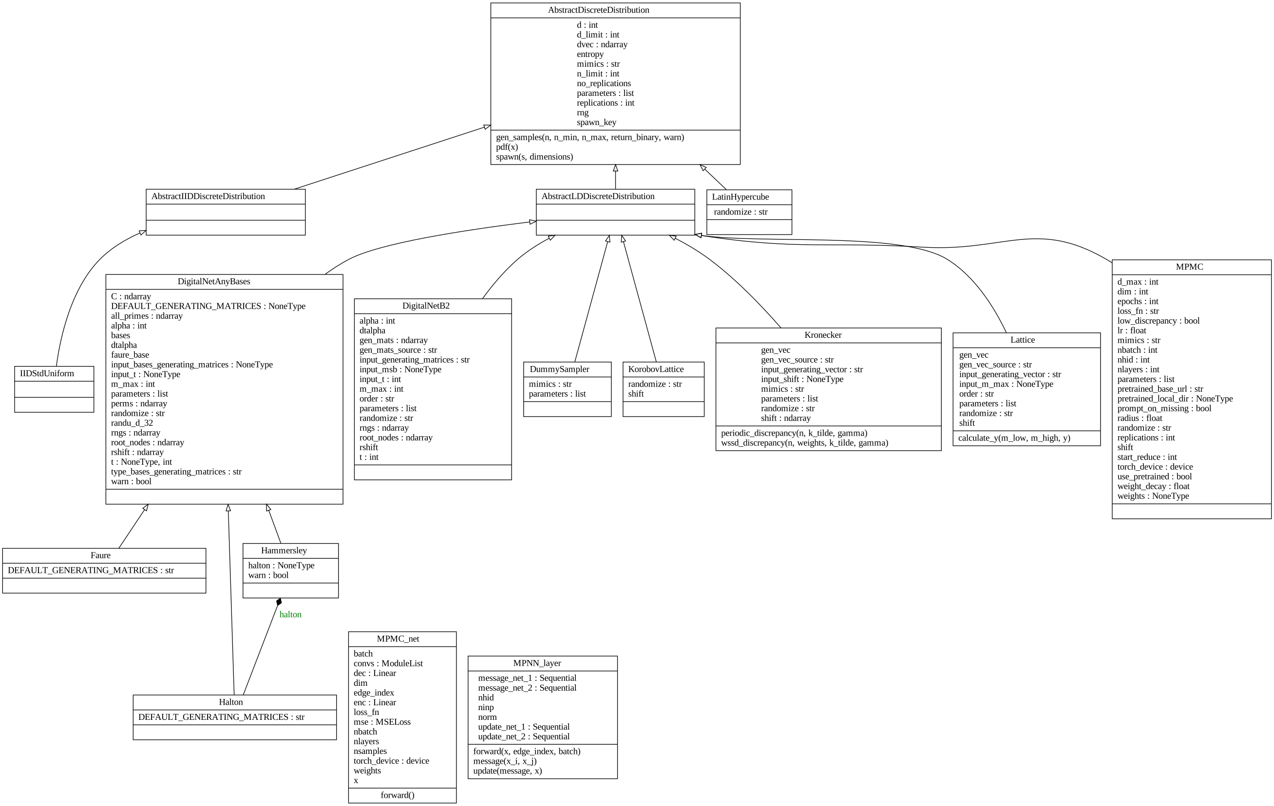
UML Overview

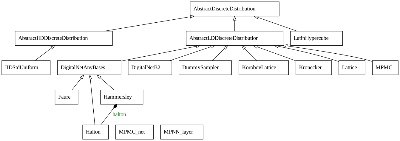
`AbstractDiscreteDistribution`

Bases: object

Source code in qmcpy/discrete_distribution/abstract_discrete_distribution.py

def __init__(self, dimension, replications, seed, d_limit, n_limit):
    self.mimics = "StdUniform"
    if not hasattr(self, "parameters"):
        self.parameters = []
    self.d_limit = d_limit
    self.n_limit = n_limit
    if not (
        np.isscalar(self.d_limit)
        and self.d_limit > 0
        and np.isscalar(self.n_limit)
        and self.n_limit > 0
    ):
        raise ParameterError("d_limit and n_limit must be greater than 0")
    self.d_limit = np.inf if self.d_limit == np.inf else int(self.d_limit)
    self.n_limit = np.inf if self.n_limit == np.inf else int(self.n_limit)
    self.no_replications = replications is None
    self.replications = 1 if self.no_replications else int(replications)
    if self.replications < 0:
        raise ParameterError("replications must be None or a postive int")
    if (
        isinstance(dimension, list)
        or isinstance(dimension, tuple)
        or isinstance(dimension, np.ndarray)
    ):
        self.dvec = np.array(dimension, dtype=int)
        self.d = len(self.dvec)
        if not (self.dvec.ndim == 1 and len(np.unique(self.dvec)) == self.d):
            raise ParameterError("dimension must be a 1d array of unique values")
    else:
        self.d = int(dimension)
        self.dvec = np.arange(self.d)
    if any(self.dvec > self.d_limit):
        raise ParameterError(
            "dimension greater than dimension limit %d" % self.d_limit
        )
    self._base_seed = (
        seed
        if isinstance(seed, np.random.SeedSequence)
        else np.random.SeedSequence(seed)
    )
    self.entropy = self._base_seed.entropy
    self.spawn_key = self._base_seed.spawn_key
    self.rng = np.random.Generator(np.random.SFC64(self._base_seed))

call

__call__(n=None, n_min=None, n_max=None, return_binary=False, warn=True)

If just n is supplied, generate samples from the sequence at indices 0,...,n-1.
If n_min and n_max are supplied, generate samples from the sequence at indices n_min,...,n_max-1.
If n and n_min are supplied, then generate samples from the sequence at indices n,...,n_min-1.

Parameters:

Name	Type	Description	Default
`n`	`Union[None, int]`	Number of points to generate.	`None`
`n_min`	`Union[None, int]`	Starting index of sequence.	`None`
`n_max`	`Union[None, int]`	Final index of sequence.	`None`
`return_binary`	`bool`	Only used for `DigitalNetB2`. If `True`, only return the integer representation `x_integer` of base 2 digital net.	`False`
`warn`	`bool`	If `False`, disable warnings when generating samples.	`True`

Returns:

Name	Type	Description
`x`	`ndarray`	Samples from the sequence. If `replications` is `None` then this will be of size (`n_max`-`n_min`) $\times$ `dimension` If `replications` is a positive int, then `x` will be of size `replications` $\times$ (`n_max`-`n_min`) $\times$ `dimension` Note that if `return_binary=True` then `x` is returned where `x` are integer representations of the digital net points.

Source code in qmcpy/discrete_distribution/abstract_discrete_distribution.py

def __call__(self, n=None, n_min=None, n_max=None, return_binary=False, warn=True):
    r"""
    - If just `n` is supplied, generate samples from the sequence at indices 0,...,`n`-1.
    - If `n_min` and `n_max` are supplied, generate samples from the sequence at indices `n_min`,...,`n_max`-1.
    - If `n` and `n_min` are supplied, then generate samples from the sequence at indices `n`,...,`n_min`-1.

    Args:
        n (Union[None, int]): Number of points to generate.
        n_min (Union[None, int]): Starting index of sequence.
        n_max (Union[None, int]): Final index of sequence.
        return_binary (bool): Only used for `DigitalNetB2`.
            If `True`, *only* return the integer representation `x_integer` of base 2 digital net.
        warn (bool): If `False`, disable warnings when generating samples.

    Returns:
        x (np.ndarray): Samples from the sequence.

            - If `replications` is `None` then this will be of size (`n_max`-`n_min`) $\times$ `dimension`
            - If `replications` is a positive int, then `x` will be of size `replications` $\times$ (`n_max`-`n_min`) $\times$ `dimension`

            Note that if `return_binary=True` then `x` is returned where `x` are integer representations of the digital net points.
    """
    return self.gen_samples(
        n=n, n_min=n_min, n_max=n_max, return_binary=return_binary, warn=warn
    )

spawn

spawn(s=1, dimensions=None)

Spawn new instances of the current discrete distribution but with new seeds and dimensions. Used by multi-level QMC algorithms which require different seeds and dimensions on each level.

Note

Use replications instead of using spawn when possible, e.g., when spawning copies which all have the same dimension.

Parameters:

Name	Type	Description	Default
`s`	`int`	Number of copies to spawn	`1`
`dimensions`	`ndarray`	Length `s` array of dimensions for each copy. Defaults to the current dimension.	`None`

Returns:

Name	Type	Description
`spawned_discrete_distribs`	`list`	Discrete distributions with new seeds and dimensions.

Source code in qmcpy/discrete_distribution/abstract_discrete_distribution.py

def spawn(self, s=1, dimensions=None):
    r"""
    Spawn new instances of the current discrete distribution but with new seeds and dimensions.
    Used by multi-level QMC algorithms which require different seeds and dimensions on each level.

    Note:
        Use `replications` instead of using `spawn` when possible, e.g., when spawning copies which all have the same dimension.

    Args:
        s (int): Number of copies to spawn
        dimensions (np.ndarray): Length `s` array of dimensions for each copy. Defaults to the current dimension.

    Returns:
        spawned_discrete_distribs (list): Discrete distributions with new seeds and dimensions.
    """
    s = int(s)
    if s <= 0:
        raise ParameterError("Must spawn s>0 instances")
    if dimensions is None:
        dimensions = np.tile(self.d, s)
    elif (
        isinstance(dimensions, list)
        or isinstance(dimensions, tuple)
        or isinstance(dimensions, np.ndarray)
    ):
        dimensions = np.array(dimensions, dtype=int)
    else:
        dimensions = np.tile(dimensions, s)
    if not (dimensions.ndim == 1 and len(dimensions) == s):
        raise ParameterError("dimensions must be a length s np.ndarray")
    child_seeds = self._base_seed.spawn(s)
    spawned_discrete_distribs = [
        self._spawn(child_seeds[i], int(dimensions[i])) for i in range(s)
    ]
    return spawned_discrete_distribs

`DigitalNetB2`

Bases: AbstractLDDiscreteDistribution

Low discrepancy digital net in base 2.

Note

Digital net sample sizes should be powers of $2$ e.g. $1$, $2$, $4$, $8$, $16$, $\dots$.
The first point of an unrandomized digital nets is the origin.
Sobol is an alias for DigitalNetB2.
To use higher order digital nets, either:
- Pass in generating_matrices without interlacing and supply alpha>1 to apply interlacing, or
- Pass in generating_matrices with interlacing and set alpha=1 to avoid additional interlacing
i.e. do not pass in interlaced generating_matrices and set alpha>1, this will apply additional interlacing.

Examples:

>>> discrete_distrib = DigitalNetB2(2,seed=7)
>>> discrete_distrib(4)
array([[0.72162356, 0.914955  ],
       [0.16345554, 0.42964856],
       [0.98676255, 0.03436384],
       [0.42956655, 0.55876342]])
>>> discrete_distrib(1) # first point in the sequence
array([[0.72162356, 0.914955  ]])
>>> discrete_distrib
DigitalNetB2 (AbstractLDDiscreteDistribution)
    d               2^(1)
    replications    1
    randomize       LMS DS
    gen_mats_source joe_kuo.6.21201.txt
    order           RADICAL INVERSE
    t               63
    alpha           1
    n_limit         2^(32)
    entropy         7

Replications of independent randomizations

>>> x = DigitalNetB2(dimension=3,seed=7,replications=2)(4)
>>> x.shape
(2, 4, 3)
>>> x
array([[[0.24653277, 0.1821862 , 0.74732591],
        [0.68152903, 0.66169442, 0.42891961],
        [0.48139855, 0.79818233, 0.08201287],
        [0.91541325, 0.29520621, 0.77495809]],

       [[0.44876891, 0.85899604, 0.50549679],
        [0.53635924, 0.04353443, 0.33564946],
        [0.23214143, 0.29281506, 0.06841036],
        [0.75295715, 0.60241448, 0.76962976]]])

Different orderings (avoid warnings that the first point is the origin)

>>> DigitalNetB2(dimension=2,randomize=False,order="GRAY")(n_min=2,n_max=4,warn=False)
array([[0.75, 0.25],
       [0.25, 0.75]])
>>> DigitalNetB2(dimension=2,randomize=False,order="RADICAL INVERSE")(n_min=2,n_max=4,warn=False)
array([[0.25, 0.75],
       [0.75, 0.25]])

Generating matrices from https://github.com/QMCSoftware/LDData/tree/main/dnet

>>> DigitalNetB2(dimension=3,randomize=False,generating_matrices="mps.nx_s5_alpha2_m32.txt")(8,warn=False)
array([[0.        , 0.        , 0.        ],
       [0.75841841, 0.45284834, 0.48844557],
       [0.57679828, 0.13226272, 0.10061957],
       [0.31858402, 0.32113875, 0.39369111],
       [0.90278927, 0.45867532, 0.01803333],
       [0.14542431, 0.02548793, 0.4749614 ],
       [0.45587539, 0.33081476, 0.11474426],
       [0.71318879, 0.15377192, 0.37629925]])

All randomizations

>>> DigitalNetB2(dimension=3,randomize='LMS DS',seed=5)(8)
array([[0.69346401, 0.20118185, 0.64779396],
       [0.43998032, 0.90102467, 0.0936172 ],
       [0.86663563, 0.60910036, 0.26043276],
       [0.11327376, 0.30772653, 0.93959283],
       [0.62102883, 0.79169756, 0.77051637],
       [0.37451038, 0.1231324 , 0.46634012],
       [0.94785596, 0.38577413, 0.13377215],
       [0.20121617, 0.71843325, 0.56293458]])
>>> DigitalNetB2(dimension=3,randomize='LMS',seed=5)(8,warn=False)
array([[0.        , 0.        , 0.        ],
       [0.75446077, 0.83265937, 0.69584079],
       [0.42329494, 0.65793842, 0.90427279],
       [0.67763292, 0.48937304, 0.33344964],
       [0.18550714, 0.97332905, 0.3772791 ],
       [0.93104851, 0.17195496, 0.82311652],
       [0.26221346, 0.31742386, 0.53093284],
       [0.50787715, 0.5172669 , 0.2101083 ]])
>>> DigitalNetB2(dimension=3,randomize='DS',seed=5)(8)
array([[0.68383949, 0.04047995, 0.42903182],
       [0.18383949, 0.54047995, 0.92903182],
       [0.93383949, 0.79047995, 0.67903182],
       [0.43383949, 0.29047995, 0.17903182],
       [0.55883949, 0.66547995, 0.05403182],
       [0.05883949, 0.16547995, 0.55403182],
       [0.80883949, 0.41547995, 0.80403182],
       [0.30883949, 0.91547995, 0.30403182]])
>>> DigitalNetB2(dimension=3,randomize='OWEN',seed=5)(8)
array([[0.33595486, 0.05834975, 0.30066401],
       [0.89110875, 0.84905188, 0.81833285],
       [0.06846074, 0.59997956, 0.67064205],
       [0.6693703 , 0.25824002, 0.10469644],
       [0.44586618, 0.99161977, 0.1873488 ],
       [0.84245267, 0.16445553, 0.56544372],
       [0.18546359, 0.44859876, 0.97389524],
       [0.61215442, 0.64341386, 0.44529863]])

Higher order net without randomization

>>> DigitalNetB2(dimension=3,randomize='FALSE',seed=7,alpha=2)(4,warn=False)
array([[0.    , 0.    , 0.    ],
       [0.75  , 0.75  , 0.75  ],
       [0.4375, 0.9375, 0.1875],
       [0.6875, 0.1875, 0.9375]])

Higher order nets with randomizations and replications

>>> DigitalNetB2(dimension=3,randomize='LMS DS',seed=7,replications=2,alpha=2)(4,warn=False)
array([[[0.42955149, 0.89149058, 0.43867111],
        [0.68701828, 0.07601148, 0.51312447],
        [0.10088033, 0.16293661, 0.25144138],
        [0.85846252, 0.87103178, 0.70041789]],

       [[0.27151905, 0.42406763, 0.21917369],
        [0.55035224, 0.67864387, 0.90033876],
        [0.19356758, 0.57589964, 0.00347701],
        [0.97235125, 0.32168581, 0.86920948]]])
>>> DigitalNetB2(dimension=3,randomize='LMS',seed=7,replications=2,alpha=2)(4,warn=False)
array([[[0.        , 0.        , 0.        ],
        [0.75817062, 0.96603053, 0.94947625],
        [0.45367986, 0.80295638, 0.18778553],
        [0.71171791, 0.2295424 , 0.76175441]],

       [[0.        , 0.        , 0.        ],
        [0.78664636, 0.75470215, 0.86876474],
        [0.45336727, 0.99953621, 0.22253579],
        [0.73996397, 0.24544824, 0.9008679 ]]])
>>> DigitalNetB2(dimension=3,randomize='DS',seed=7,replications=2,alpha=2)(4)
array([[[0.04386058, 0.58727432, 0.3691824 ],
        [0.79386058, 0.33727432, 0.6191824 ],
        [0.48136058, 0.39977432, 0.4316824 ],
        [0.73136058, 0.64977432, 0.6816824 ]],

       [[0.65212985, 0.69669968, 0.10605352],
        [0.40212985, 0.44669968, 0.85605352],
        [0.83962985, 0.25919968, 0.16855352],
        [0.08962985, 0.50919968, 0.91855352]]])
>>> DigitalNetB2(dimension=3,randomize='OWEN',seed=7,replications=2,alpha=2)(4)
array([[[0.46368517, 0.03964427, 0.62172094],
        [0.7498683 , 0.76141348, 0.4243043 ],
        [0.01729754, 0.97968459, 0.65963223],
        [0.75365329, 0.1903774 , 0.34141493]],

       [[0.52252547, 0.5679709 , 0.05949112],
        [0.27248656, 0.36488289, 0.81844058],
        [0.94219959, 0.39172304, 0.20285965],
        [0.19716391, 0.64741585, 0.92494554]]])

References:

Marius Hofert and Christiane Lemieux. qrng: (Randomized) Quasi-Random Number Generators (2019). R package version 0.0-7. https://CRAN.R-project.org/package=qrng.
Faure, Henri, and Christiane Lemieux. Implementation of Irreducible Sobol' Sequences in Prime Power Bases. Mathematics and Computers in Simulation 161 (2019): 13-22. Crossref. Web.
F.Y. Kuo, D. Nuyens. Application of quasi-Monte Carlo methods to elliptic PDEs with random diffusion coefficients - a survey of analysis and implementation. Foundations of Computational Mathematics, 16(6):1631-1696, 2016. https://link.springer.com/article/10.1007/s10208-016-9329-5.
D. Nuyens. The Magic Point Shop of QMC point generators and generating vectors. MATLAB and Python software, 2018. https://people.cs.kuleuven.be/~dirk.nuyens/.
R. Cools, F.Y. Kuo, D. Nuyens. Constructing embedded lattice rules for multivariate integration. SIAM J. Sci. Comput., 28(6), 2162-2188.
I.M. Sobol', V.I. Turchaninov, Yu.L. Levitan, B.V. Shukhman. Quasi-Random Sequence Generators. Keldysh Institute of Applied Mathematics. Russian Academy of Sciences, Moscow (1992).
Sobol, Ilya & Asotsky, Danil & Kreinin, Alexander & Kucherenko, Sergei. (2011). Construction and Comparison of High-Dimensional Sobol' Generators. Wilmott. 2011. 10.1002/wilm.10056.
Paul Bratley and Bennett L. Fox. Algorithm 659: Implementing Sobol's quasirandom sequence generator. ACM Trans. Math. Softw. 14, 1 (March 1988), 88-100. 1988. https://doi.org/10.1145/42288.214372.

Parameters:

Name	Type	Description	Default
`dimension`	`Union[int, ndarray]`	Dimension of the generator. If an `int` is passed in, use generating vector components at indices 0,...,`dimension`-1. If an `np.ndarray` is passed in, use generating vector components at these indices.	`1`
`replications`	`int`	Number of independent randomizations of a pointset.	`None`
`seed`	`Union[None, int, np.random.SeedSeq`	Seed the random number generator for reproducibility.	`None`
`randomize`	`str`	Options are `'LMS DS'`: Linear matrix scramble with digital shift. `'LMS'`: Linear matrix scramble only. `'DS'`: Digital shift only. `'NUS'`: Nested uniform scrambling. Also known as Owen scrambling. `'FALSE'`: No randomization. In this case the first point will be the origin.	`'LMS DS'`
`generating_matrices`	`Union[str, ndarray, int]`	Specify the generating matrices. A `str` should be the name (or path) of a file from the LDData repo at https://github.com/QMCSoftware/LDData/tree/main/dnet. An `np.ndarray` of integers with shape $(d,m_\mathrm{max})$ or $(r,d,m_\mathrm{max})$ where $d$ is the number of dimensions, $r$ is the number of replications, and $2^{m_\mathrm{max}}$ is the maximum number of supported points. Setting `msb=False` will flip the bits of ints in the generating matrices.	`'joe_kuo.6.21201.txt'`
`order`	`str`	`'RADICAL INVERSE'`, or `'GRAY'` ordering. See the doctest example above.	`'RADICAL INVERSE'`
`t`	`int`	Number of bits in integer represetation of points after randomization. The number of bits in the generating matrices is inferred based on the largest value.	`63`
`alpha`	`int`	Interlacing factor for higher order nets. When `alpha`>1, interlacing is performed regardless of the generating matrices, i.e., for `alpha`>1 do not pass in generating matrices which are already interlaced. The Note for this class contains more info.	`1`
`msb`	`bool`	Flag for Most Significant Bit (MSB) vs Least Significant Bit (LSB) integer representations in generating matrices. If `msb=False` (LSB order), then integers in generating matrices will be bit-reversed.	`None`
`_verbose`	`bool`	If `True`, print linear matrix scrambling matrices.	`False`

Source code in qmcpy/discrete_distribution/digital_net_b2/digital_net_b2.py

def __init__(
    self,
    dimension=1,
    replications=None,
    seed=None,
    randomize="LMS DS",
    generating_matrices="joe_kuo.6.21201.txt",
    order="RADICAL INVERSE",
    t=63,
    alpha=1,
    msb=None,
    _verbose=False,
    # deprecated
    graycode=None,
    t_max=None,
    t_lms=None,
):
    r"""
    Args:
        dimension (Union[int, np.ndarray]): Dimension of the generator.

            - If an `int` is passed in, use generating vector components at indices 0,...,`dimension`-1.
            - If an `np.ndarray` is passed in, use generating vector components at these indices.

        replications (int): Number of independent randomizations of a pointset.
        seed (Union[None, int, np.random.SeedSeq): Seed the random number generator for reproducibility.
        randomize (str): Options are

            - `'LMS DS'`: Linear matrix scramble with digital shift.
            - `'LMS'`: Linear matrix scramble only.
            - `'DS'`: Digital shift only.
            - `'NUS'`: Nested uniform scrambling. Also known as Owen scrambling.
            - `'FALSE'`: No randomization. In this case the first point will be the origin.

        generating_matrices (Union[str, np.ndarray, int]): Specify the generating matrices.

            - A `str` should be the name (or path) of a file from the LDData repo at [https://github.com/QMCSoftware/LDData/tree/main/dnet](https://github.com/QMCSoftware/LDData/tree/main/dnet).
            - An `np.ndarray` of integers with shape $(d,m_\mathrm{max})$ or $(r,d,m_\mathrm{max})$ where $d$ is the number of dimensions, $r$ is the number of replications, and $2^{m_\mathrm{max}}$ is the maximum number of supported points. Setting `msb=False` will flip the bits of ints in the generating matrices.

        order (str): `'RADICAL INVERSE'`, or `'GRAY'` ordering. See the doctest example above.
        t (int): Number of bits in integer represetation of points *after* randomization. The number of bits in the generating matrices is inferred based on the largest value.
        alpha (int): Interlacing factor for higher order nets.
            When `alpha`>1, interlacing is performed regardless of the generating matrices,
            i.e., for `alpha`>1 do *not* pass in generating matrices which are already interlaced.
            The Note for this class contains more info.
        msb (bool): Flag for Most Significant Bit (MSB) vs Least Significant Bit (LSB) integer representations in generating matrices. If `msb=False` (LSB order), then integers in generating matrices will be bit-reversed.
        _verbose (bool): If `True`, print linear matrix scrambling matrices.
    """
    if graycode is not None:
        order = "GRAY" if graycode else "RADICAL INVERSE"
        warnings.warn(
            "graycode argument deprecated, set order='GRAY' or order='RADICAL INVERSE' instead. Using order='%s'"
            % order,
            ParameterWarning,
        )
    if t_lms is not None:
        t = t_lms
        warnings.warn(
            "t_lms argument deprecated. Set t instead. Using t = %d" % t,
            ParameterWarning,
        )
    if t_max is not None:
        warnings.warn(
            "t_max is deprecated as it can be inferred from the generating matrices. Set t to change the number of bits after randomization.",
            ParameterWarning,
        )
    self.parameters = [
        "randomize",
        "gen_mats_source",
        "order",
        "t",
        "alpha",
        "n_limit",
    ]
    self.input_generating_matrices = deepcopy(generating_matrices)
    self.input_t = deepcopy(t)
    self.input_msb = deepcopy(msb)
    if (
        isinstance(generating_matrices, str)
        and generating_matrices == "joe_kuo.6.21201.txt"
    ):
        self.gen_mats_source = generating_matrices
        if np.isscalar(dimension) and dimension <= 1024 and alpha == 1:
            gen_mats = np.load(
                dirname(abspath(__file__))
                + "/generating_matrices/joe_kuo.6.1024.npy"
            )[None, :]
            d_limit = 1024
        else:
            gen_mats = np.load(
                dirname(abspath(__file__))
                + "/generating_matrices/joe_kuo.6.21201.npy"
            )[None, :]
            d_limit = 21201
        msb = True
        n_limit = 4294967296
        self._t_curr = 32
        compat_shift = self._t_curr - t if self._t_curr >= t else 0
        if compat_shift > 0:
            warnings.warn(
                "Truncating ints in generating matrix to have t = %d bits." % t,
                ParameterWarning,
            )
        gen_mats = gen_mats >> compat_shift
    elif isinstance(generating_matrices, str):
        self.gen_mats_source = generating_matrices
        assert generating_matrices[-4:] == ".txt"
        local_root = dirname(abspath(__file__)) + "/generating_matrices/"
        repos = DataSource()
        if repos.exists(local_root + generating_matrices):
            datafile = repos.open(local_root + generating_matrices)
        elif repos.exists(
            "https://raw.githubusercontent.com/QMCSoftware/LDData/refs/heads/main/dnet/"
            + generating_matrices
        ):
            datafile = repos.open(
                "https://raw.githubusercontent.com/QMCSoftware/LDData/refs/heads/main/dnet/"
                + generating_matrices
            )
        elif repos.exists(
            "https://raw.githubusercontent.com/QMCSoftware/LDData/refs/heads/main/"
            + generating_matrices
        ):
            datafile = repos.open(
                "https://raw.githubusercontent.com/QMCSoftware/LDData/refs/heads/main/"
                + generating_matrices
            )
        elif repos.exists(
            "https://raw.githubusercontent.com/QMCSoftware/LDData/refs/heads/main/dnet/"
            + generating_matrices[7:]
        ):
            datafile = repos.open(
                "https://raw.githubusercontent.com/QMCSoftware/LDData/refs/heads/main/dnet/"
                + generating_matrices[7:]
            )
        elif repos.exists(
            "https://raw.githubusercontent.com/QMCSoftware/" + generating_matrices
        ):
            datafile = repos.open(
                "https://raw.githubusercontent.com/QMCSoftware/"
                + generating_matrices
            )
        elif repos.exists(generating_matrices):
            datafile = repos.open(generating_matrices)
        else:
            raise ParameterError("LDData path %s not found" % generating_matrices)
        contents = [line.rstrip("\n").strip() for line in datafile.readlines()]
        contents = [line.split("#", 1)[0] for line in contents if line[0] != "#"]
        datafile.close()
        msb = True
        assert int(contents[0]) == 2, "DigitalNetB2 requires base=2 "  # base 2
        d_limit = int(contents[1])
        n_limit = int(contents[2])
        self._t_curr = int(contents[3])
        compat_shift = self._t_curr - t if self._t_curr >= t else 0
        if compat_shift > 0:
            warnings.warn(
                "Truncating ints in generating matrix to have t = %d bits." % t,
                ParameterWarning,
            )
        gen_mats = np.array(
            [
                [int(v) >> compat_shift for v in line.split(" ")]
                for line in contents[4:]
            ],
            dtype=np.uint64,
        )[None, :]
    elif isinstance(generating_matrices, np.ndarray):
        self.gen_mats_source = "custom"
        assert generating_matrices.ndim == 2 or generating_matrices.ndim == 3
        gen_mats = (
            generating_matrices[None, :, :]
            if generating_matrices.ndim == 2
            else generating_matrices
        )
        assert isinstance(
            msb, bool
        ), "when generating_matrices is a np.ndarray you must set either msb=True (for most significant bit ordering) or msb=False (for least significant bit ordering which will require a bit reversal)"
        gen_mat_max = gen_mats.max()
        assert gen_mat_max > 0, "generating matrix must have positive ints"
        self._t_curr = int(np.ceil(np.log2(gen_mat_max + 1)))
        d_limit = gen_mats.shape[1]
        n_limit = int(2 ** (gen_mats.shape[2]))
    else:
        raise ParameterError(
            "invalid generating_matrices, must be a string or np.ndarray."
        )
    super(DigitalNetB2, self).__init__(
        dimension, replications, seed, d_limit, n_limit
    )
    assert (
        gen_mats.ndim == 3
        and gen_mats.shape[1] >= self.d
        and (gen_mats.shape[0] == 1 or gen_mats.shape[0] == self.replications)
        and gen_mats.shape[2] > 0
    ), "invalid gen_mats.shape = %s" % str(gen_mats.shape)
    self.m_max = int(gen_mats.shape[-1])
    if isinstance(generating_matrices, np.ndarray) and (not msb):
        qmctoolscl.dnb2_gmat_lsb_to_msb(
            np.uint64(gen_mats.shape[0]),
            np.uint64(self.d),
            np.uint64(self.m_max),
            np.tile(np.uint64(self._t_curr), int(gen_mats.shape[0])),
            gen_mats,
            gen_mats,
            backend="c",
        )
    self.order = str(order).upper().strip().replace("_", " ")
    if self.order == "GRAY CODE":
        self.order = "GRAY"
    if self.order == "NATURAL":
        self.order = "RADICAL INVERSE"
    assert self.order in ["RADICAL INVERSE", "GRAY"]
    assert isinstance(t, int) and t > 0
    assert self._t_curr <= t <= 64, (
        "t must no more than 64 and no less than %d (the number of bits used to represent the generating matrices)"
        % (self._t_curr)
    )
    assert isinstance(alpha, int) and alpha > 0
    self.alpha = alpha
    if self.alpha > 1:
        assert (
            self.dvec == np.arange(self.d)
        ).all(), "digital interlacing requires dimension is an int"
        if self.m_max != self._t_curr:
            warnings.warn(
                "Digital interlacing is often performed on matrices with the number of columns (m_max = %d) equal to the number of bits in each int (%d), but this is not the case. Ensure you are NOT setting alpha>1 when generating matrices are already interlaced."
                % (self.m_max, self._t_curr),
                ParameterWarning,
            )
    self._verbose = _verbose
    self.randomize = str(randomize).upper().strip().replace("_", " ")
    if self.randomize == "TRUE":
        self.randomize = "LMS DS"
    if self.randomize == "OWEN":
        self.randomize = "NUS"
    if self.randomize == "NONE":
        self.randomize = "FALSE"
    if self.randomize == "NO":
        self.randomize = "FALSE"
    assert self.randomize in ["LMS DS", "LMS", "DS", "NUS", "FALSE"]
    self.dtalpha = self.alpha * self.d
    if self.randomize == "FALSE":
        if self.alpha == 1:
            self.gen_mats = gen_mats[:, self.dvec, :]
            self.t = self._t_curr
        else:
            t_alpha = min(self.alpha * self._t_curr, t)
            gen_mat_ho = np.empty(
                (gen_mats.shape[0], self.d, self.m_max), dtype=np.uint64
            )
            qmctoolscl.dnb2_interlace(
                np.uint64(gen_mats.shape[0]),
                np.uint64(self.d),
                np.uint64(self.m_max),
                np.uint64(self.dtalpha),
                np.uint64(self._t_curr),
                np.uint64(t_alpha),
                np.uint64(self.alpha),
                gen_mats[:, : self.dtalpha, :].copy(),
                gen_mat_ho,
                backend="c",
            )
            self.gen_mats = gen_mat_ho
            self._t_curr = t_alpha
            self.t = self._t_curr
    elif self.randomize == "DS":
        if self.alpha == 1:
            self.gen_mats = gen_mats[:, self.dvec, :]
            self.t = t
        else:
            t_alpha = min(self.alpha * self._t_curr, t)
            gen_mat_ho = np.empty(
                (gen_mats.shape[0], self.d, self.m_max), dtype=np.uint64
            )
            qmctoolscl.dnb2_interlace(
                np.uint64(gen_mats.shape[0]),
                np.uint64(self.d),
                np.uint64(self.m_max),
                np.uint64(self.dtalpha),
                np.uint64(self._t_curr),
                np.uint64(t_alpha),
                np.uint64(self.alpha),
                gen_mats[:, : self.dtalpha, :].copy(),
                gen_mat_ho,
                backend="c",
            )
            self.gen_mats = gen_mat_ho
            self._t_curr = t_alpha
            self.t = t
        self.rshift = qmctoolscl.random_tbit_uint64s(
            self.rng, self.t, (self.replications, self.d)
        )
    elif self.randomize in ["LMS", "LMS DS"]:
        if self.alpha == 1:
            gen_mat_lms = np.empty(
                (self.replications, self.d, self.m_max), dtype=np.uint64
            )
            S = qmctoolscl.dnb2_get_linear_scramble_matrix(
                self.rng,
                np.uint64(self.replications),
                np.uint64(self.d),
                np.uint64(self._t_curr),
                np.uint64(t),
                np.uint64(self._verbose),
            )
            qmctoolscl.dnb2_linear_matrix_scramble(
                np.uint64(self.replications),
                np.uint64(self.d),
                np.uint64(self.m_max),
                np.uint64(gen_mats.shape[0]),
                np.uint64(t),
                S,
                gen_mats[:, self.dvec, :].copy(),
                gen_mat_lms,
                backend="c",
            )
            self.gen_mats = gen_mat_lms
            self._t_curr = t
            self.t = self._t_curr
        else:
            gen_mat_lms = np.empty(
                (self.replications, self.dtalpha, self.m_max), dtype=np.uint64
            )
            S = qmctoolscl.dnb2_get_linear_scramble_matrix(
                self.rng,
                np.uint64(self.replications),
                np.uint64(self.dtalpha),
                np.uint64(self._t_curr),
                np.uint64(t),
                np.uint64(self._verbose),
            )
            qmctoolscl.dnb2_linear_matrix_scramble(
                np.uint64(self.replications),
                np.uint64(self.dtalpha),
                np.uint64(self.m_max),
                np.uint64(gen_mats.shape[0]),
                np.uint64(t),
                S,
                gen_mats[:, : self.dtalpha, :].copy(),
                gen_mat_lms,
                backend="c",
            )
            gen_mat_lms_ho = np.empty(
                (self.replications, self.d, self.m_max), dtype=np.uint64
            )
            qmctoolscl.dnb2_interlace(
                np.uint64(self.replications),
                np.uint64(self.d),
                np.uint64(self.m_max),
                np.uint64(self.dtalpha),
                np.uint64(t),
                np.uint64(t),
                np.uint64(self.alpha),
                gen_mat_lms,
                gen_mat_lms_ho,
                backend="c",
            )
            self.gen_mats = gen_mat_lms_ho
            self._t_curr = t
            self.t = self._t_curr
        if self.randomize == "LMS DS":
            self.rshift = qmctoolscl.random_tbit_uint64s(
                self.rng, self.t, (self.replications, self.d)
            )
    elif self.randomize == "NUS":
        if alpha == 1:
            new_seeds = self._base_seed.spawn(self.replications * self.d)
            self.rngs = np.array(
                [
                    np.random.Generator(np.random.SFC64(new_seeds[j]))
                    for j in range(self.replications * self.d)
                ]
            ).reshape(self.replications, self.d)
            self.root_nodes = np.array(
                [
                    qmctoolscl.NUSNode_dnb2()
                    for i in range(self.replications * self.d)
                ]
            ).reshape(self.replications, self.d)
            self.gen_mats = gen_mats[:, self.dvec, :].copy()
            self.t = t
        else:
            self.dtalpha = self.alpha * self.d
            new_seeds = self._base_seed.spawn(self.replications * self.dtalpha)
            self.rngs = np.array(
                [
                    np.random.Generator(np.random.SFC64(new_seeds[j]))
                    for j in range(self.replications * self.dtalpha)
                ]
            ).reshape(self.replications, self.dtalpha)
            self.root_nodes = np.array(
                [
                    qmctoolscl.NUSNode_dnb2()
                    for i in range(self.replications * self.dtalpha)
                ]
            ).reshape(self.replications, self.dtalpha)
            self.gen_mats = gen_mats[:, : self.dtalpha, :].copy()
            self.t = t
    else:
        raise ParameterError("self.randomize parsing error")
    self.gen_mats = np.ascontiguousarray(self.gen_mats)
    gen_mat_max = self.gen_mats.max()
    assert gen_mat_max > 0, "generating matrix must have positive ints"
    assert self._t_curr == int(np.ceil(np.log2(gen_mat_max + 1)))
    assert (
        0 < self._t_curr <= self.t <= 64
    ), "invalid 0 <= self._t_curr (%d) <= self.t (%d) <= 64" % (
        self._t_curr,
        self.t,
    )
    if self.randomize == "FALSE":
        assert self.gen_mats.shape[0] == self.replications, (
            "randomize='FALSE' but replications = %d does not equal the number of sets of generating matrices %d"
            % (self.replications, self.gen_mats.shape[0])
        )

`Lattice`

Bases: AbstractLDDiscreteDistribution

Low discrepancy lattice sequence.

Note

Lattice sample sizes should be powers of $2$ e.g. $1$, $2$, $4$, $8$, $16$, $\dots$.
The first point of an unrandomized lattice is the origin.

Examples:

>>> discrete_distrib = Lattice(2,seed=7)
>>> discrete_distrib(4)
array([[0.04386058, 0.58727432],
       [0.54386058, 0.08727432],
       [0.29386058, 0.33727432],
       [0.79386058, 0.83727432]])
>>> discrete_distrib(1) # first point in the sequence
array([[0.04386058, 0.58727432]])
>>> discrete_distrib
Lattice (AbstractLDDiscreteDistribution)
    d               2^(1)
    replications    1
    randomize       SHIFT
    gen_vec_source  kuo.lattice-33002-1024-1048576.9125.txt
    order           RADICAL INVERSE
    n_limit         2^(20)
    entropy         7

Replications of independent randomizations

>>> x = Lattice(3,seed=7,replications=2)(4)
>>> x.shape
(2, 4, 3)
>>> x
array([[[0.04386058, 0.58727432, 0.3691824 ],
        [0.54386058, 0.08727432, 0.8691824 ],
        [0.29386058, 0.33727432, 0.1191824 ],
        [0.79386058, 0.83727432, 0.6191824 ]],

       [[0.65212985, 0.69669968, 0.10605352],
        [0.15212985, 0.19669968, 0.60605352],
        [0.90212985, 0.44669968, 0.85605352],
        [0.40212985, 0.94669968, 0.35605352]]])

Different orderings (avoid warnings that the first point is the origin).

>>> Lattice(dimension=2,randomize=False,order='RADICAL INVERSE')(4,warn=False)
array([[0.  , 0.  ],
       [0.5 , 0.5 ],
       [0.25, 0.75],
       [0.75, 0.25]])
>>> Lattice(dimension=2,randomize=False,order='GRAY')(4,warn=False)
array([[0.  , 0.  ],
       [0.5 , 0.5 ],
       [0.75, 0.25],
       [0.25, 0.75]])
>>> Lattice(dimension=2,randomize=False,order='LINEAR')(4,warn=False)
array([[0.  , 0.  ],
       [0.25, 0.75],
       [0.5 , 0.5 ],
       [0.75, 0.25]])

Generating vector from https://github.com/QMCSoftware/LDData/tree/main/lattice

>>> Lattice(dimension=3,randomize=False,generating_vector="mps.exod2_base2_m20_CKN.txt")(8,warn=False)
array([[0.   , 0.   , 0.   ],
       [0.5  , 0.5  , 0.5  ],
       [0.25 , 0.75 , 0.75 ],
       [0.75 , 0.25 , 0.25 ],
       [0.125, 0.375, 0.375],
       [0.625, 0.875, 0.875],
       [0.375, 0.125, 0.125],
       [0.875, 0.625, 0.625]])

Random generating vector supporting $2^{25}$ points

>>> discrete_distrib = Lattice(3,generating_vector=25,seed=55,randomize=False)
>>> discrete_distrib.gen_vec
array([[       1, 11961679, 12107519]], dtype=uint64)
>>> discrete_distrib(4,warn=False)
array([[0.  , 0.  , 0.  ],
       [0.5 , 0.5 , 0.5 ],
       [0.25, 0.75, 0.75],
       [0.75, 0.25, 0.25]])

Two random generating vectors both supporting $2^{25}$ points along with independent random shifts

>>> discrete_distrib = Lattice(3,seed=7,generating_vector=25,replications=2)
>>> discrete_distrib.gen_vec
array([[       1, 32809149,  1471719],
       [       1,   275319, 19705657]], dtype=uint64)
>>> discrete_distrib(4)
array([[[0.3691824 , 0.65212985, 0.69669968],
        [0.8691824 , 0.15212985, 0.19669968],
        [0.6191824 , 0.90212985, 0.44669968],
        [0.1191824 , 0.40212985, 0.94669968]],

       [[0.10605352, 0.63025643, 0.13630282],
        [0.60605352, 0.13025643, 0.63630282],
        [0.35605352, 0.38025643, 0.38630282],
        [0.85605352, 0.88025643, 0.88630282]]])

References

Sou-Cheng T. Choi, Yuhan Ding, Fred J. Hickernell, Lan Jiang, Lluis Antoni Jimenez Rugama, Da Li, Jagadeeswaran Rathinavel, Xin Tong, Kan Zhang, Yizhi Zhang, and Xuan Zhou. GAIL: Guaranteed Automatic Integration Library (Version 2.3), MATLAB Software, 2019. http://gailgithub.github.io/GAIL_Dev/.
F.Y. Kuo, D. Nuyens. Application of quasi-Monte Carlo methods to elliptic PDEs with random diffusion coefficients - a survey of analysis and implementation. Foundations of Computational Mathematics, 16(6):1631-1696, 2016. https://link.springer.com/article/10.1007/s10208-016-9329-5.
D. Nuyens. The Magic Point Shop of QMC point generators and generating vectors. MATLAB and Python software, 2018. https://people.cs.kuleuven.be/~dirk.nuyens/.
R. Cools, F.Y. Kuo, D. Nuyens. Constructing embedded lattice rules for multivariate integration. SIAM J. Sci. Comput., 28(6), 2162-2188.
P. L'Ecuyer, D. Munger. LatticeBuilder: A General Software Tool for Constructing Rank-1 Lattice Rules. ACM Transactions on Mathematical Software. 42. (2015). 10.1145/2754929.

Parameters:

Name	Type	Description	Default
`dimension`	`Union[int, ndarray]`	Dimension of the generator. If an `int` is passed in, use generating vector components at indices 0,...,`dimension`-1. If an `np.ndarray` is passed in, use generating vector components at these indices.	`1`
`replications`	`int`	Number of independent randomizations.	`None`
`seed`	`Union[None, int, np.random.SeedSeq`	Seed the random number generator for reproducibility.	`None`
`randomize`	`str`	Options are `'SHIFT'`: Random shift. `'FALSE'`: No randomization. In this case the first point will be the origin.	`'SHIFT'`
`generating_vector`	`Union[str, ndarray, int]`	Specify the generating vector. A `str` should be the name (or path) of a file from the LDData repo at https://github.com/QMCSoftware/LDData/tree/main/lattice. A `np.ndarray` of integers with shape $(d,)$ or $(r,d)$ where $d$ is the number of dimensions and $r$ is the number of replications. Must supply `m_max` where $2^{m_\mathrm{max}}$ is the max number of supported samples. An `int`, call it $M$, gives the random generating vector $(1,v_1,\dots,v_{d-1})^T$ where $d$ is the dimension and $v_i$ are randomly selected from $\{3,5,\dots,2^M-1\}$ uniformly and independently. We require require $1 < M < 27$.	`'kuo.lattice-33002-1024-1048576.9125.txt'`
`order`	`str`	`'LINEAR'`, `'RADICAL INVERSE'`, or `'GRAY'` ordering. See the doctest example above.	`'RADICAL INVERSE'`
`m_max`	`int`	$2^{m_\mathrm{max}}$ is the maximum number of supported samples.	`None`

Source code in qmcpy/discrete_distribution/lattice/lattice.py

def __init__(
    self,
    dimension=1,
    replications=None,
    seed=None,
    randomize="SHIFT",
    generating_vector="kuo.lattice-33002-1024-1048576.9125.txt",
    order="RADICAL INVERSE",
    m_max=None,
):
    r"""
    Args:
        dimension (Union[int, np.ndarray]): Dimension of the generator.

            - If an `int` is passed in, use generating vector components at indices 0,...,`dimension`-1.
            - If an `np.ndarray` is passed in, use generating vector components at these indices.

        replications (int): Number of independent randomizations.
        seed (Union[None, int, np.random.SeedSeq): Seed the random number generator for reproducibility.
        randomize (str): Options are

            - `'SHIFT'`: Random shift.
            - `'FALSE'`: No randomization. In this case the first point will be the origin.

        generating_vector (Union[str, np.ndarray, int]): Specify the generating vector.

            - A `str` should be the name (or path) of a file from the LDData repo at [https://github.com/QMCSoftware/LDData/tree/main/lattice](https://github.com/QMCSoftware/LDData/tree/main/lattice).
            - A `np.ndarray` of integers with shape $(d,)$ or $(r,d)$ where $d$ is the number of dimensions and $r$ is the number of replications.
                Must supply `m_max` where $2^{m_\mathrm{max}}$ is the max number of supported samples.
            - An `int`, call it $M$,
            gives the random generating vector $(1,v_1,\dots,v_{d-1})^T$
            where $d$ is the dimension and $v_i$ are randomly selected from $\{3,5,\dots,2^M-1\}$ uniformly and independently.
            We require require $1 < M < 27$.

        order (str): `'LINEAR'`, `'RADICAL INVERSE'`, or `'GRAY'` ordering. See the doctest example above.
        m_max (int): $2^{m_\mathrm{max}}$ is the maximum number of supported samples.
    """
    self.parameters = ["randomize", "gen_vec_source", "order", "n_limit"]
    self.input_generating_vector = deepcopy(generating_vector)
    self.input_m_max = deepcopy(m_max)
    if (
        isinstance(generating_vector, str)
        and generating_vector == "kuo.lattice-33002-1024-1048576.9125.txt"
    ):
        self.gen_vec_source = generating_vector
        gen_vec = np.load(
            dirname(abspath(__file__))
            + "/generating_vectors/kuo.lattice-33002-1024-1048576.9125.npy"
        )[None, :]
        d_limit = 9125
        n_limit = 1048576
    elif isinstance(generating_vector, str):
        self.gen_vec_source = generating_vector
        assert generating_vector[-4:] == ".txt"
        local_root = dirname(abspath(__file__)) + "/generating_vectors/"
        repos = DataSource()
        if repos.exists(local_root + generating_vector):
            datafile = repos.open(local_root + generating_vector)
        elif repos.exists(
            "https://raw.githubusercontent.com/QMCSoftware/LDData/refs/heads/main/lattice/"
            + generating_vector
        ):
            datafile = repos.open(
                "https://raw.githubusercontent.com/QMCSoftware/LDData/refs/heads/main/lattice/"
                + generating_vector
            )
        elif repos.exists(
            "https://raw.githubusercontent.com/QMCSoftware/LDData/refs/heads/main/"
            + generating_vector
        ):
            datafile = repos.open(
                "https://raw.githubusercontent.com/QMCSoftware/LDData/refs/heads/main/"
                + generating_vector
            )
        elif repos.exists(
            "https://raw.githubusercontent.com/QMCSoftware/LDData/refs/heads/main/lattice/"
            + generating_vector[7:]
        ):
            datafile = repos.open(
                "https://raw.githubusercontent.com/QMCSoftware/LDData/refs/heads/main/lattice/"
                + generating_vector[7:]
            )
        elif repos.exists(
            "https://raw.githubusercontent.com/QMCSoftware/" + generating_vector
        ):
            datafile = repos.open(
                "https://raw.githubusercontent.com/QMCSoftware/" + generating_vector
            )
        elif repos.exists(generating_vector):
            datafile = repos.open(generating_vector)
        else:
            raise ParameterError("LDData path %s not found" % generating_vector)
        contents = [
            int(line.rstrip("\n").strip().split("#", 1)[0])
            for line in datafile.readlines()
            if line[0] != "#"
        ]
        datafile.close()
        d_limit = int(contents[0])
        n_limit = int(contents[1])
        gen_vec = np.array(contents[2:], dtype=np.uint64)[None, :]
    elif isinstance(generating_vector, np.ndarray):
        self.gen_vec_source = "custom"
        gen_vec = generating_vector
        if m_max is None:
            raise ParameterError(
                "m_max must be supplied when generating_vector is a np.ndarray"
            )
        n_limit = int(2**m_max)
        d_limit = int(gen_vec.shape[-1])
    elif isinstance(generating_vector, int):
        assert 1 < generating_vector < 27, "int generating vector out of range"
        n_limit = 2**generating_vector
        assert isinstance(
            dimension, int
        ), "random generating vector requires int dimension"
        d_limit = dimension
    else:
        raise ParameterError(
            "invalid generating_vector, must be a string, numpy.ndarray, or int"
        )
    super(Lattice, self).__init__(dimension, replications, seed, d_limit, n_limit)
    if isinstance(generating_vector, int):
        self.gen_vec_source = "random"
        m_max = int(np.log2(self.n_limit))
        gen_vec = np.hstack(
            [
                np.ones((self.replications, 1), dtype=np.uint64),
                2
                * self.rng.integers(
                    1,
                    2 ** (m_max - 1),
                    size=(self.replications, dimension - 1),
                    dtype=np.uint64,
                )
                + 1,
            ]
        ).copy()
    assert isinstance(gen_vec, np.ndarray)
    gen_vec = np.atleast_2d(gen_vec)
    assert (
        gen_vec.ndim == 2
        and gen_vec.shape[1] >= self.d
        and (gen_vec.shape[0] == 1 or gen_vec.shape[0] == self.replications)
    ), "invalid gen_vec.shape = %s" % str(gen_vec.shape)
    self.gen_vec = gen_vec[:, self.dvec].copy()
    self.order = str(order).upper().strip().replace("_", " ")
    if self.order == "GRAY CODE":
        self.order = "GRAY"
    if self.order == "NATURAL":
        self.order = "RADICAL INVERSE"
    assert self.order in ["LINEAR", "RADICAL INVERSE", "GRAY"]
    self.randomize = str(randomize).upper()
    if self.randomize == "TRUE":
        self.randomize = "SHIFT"
    if self.randomize == "NONE":
        self.randomize = "FALSE"
    if self.randomize == "NO":
        self.randomize = "FALSE"
    assert self.randomize in ["SHIFT", "FALSE"]
    if self.randomize == "SHIFT":
        self.shift = self.rng.uniform(size=(self.replications, self.d))
    if self.randomize == "FALSE":
        assert self.gen_vec.shape[0] == self.replications, (
            "randomize='FALSE' but replications = %d does not equal the number of sets of generating vectors %d"
            % (self.replications, self.gen_vec.shape[0])
        )

`KorobovLattice`

Bases: AbstractLDDiscreteDistribution

Korobov lattice rule with a tabulated, quality-optimized generating parameter.

A rank-1 lattice rule with $n$ points and generating vector $z\in\mathbb{Z}^d$ is $P_n(z) = \{(\{k z_1/n\},\dots,\{k z_d/n\}) : k=0,\dots,n-1\}$. The Korobov construction restricts $z$ to a single integer parameter $a$: $z(a) = (1,a,a^2,\dots,a^{d-1}) \bmod n$, with $\gcd(a,n)=1$.

Rather than searching for $a$ at construction time, this class looks up $a$ in a precomputed table, for every $(n,d)$ pair in the table, minimizing the weighted $P_2$ figure of merit (the squared worst-case integration error in the weighted Korobov space of smoothness 2) with product weights $\gamma_j = 1/j^2$.

Note

Because the optimal $a$ depends on the total number of points $n$, a Korobov lattice cannot be incrementally extended the way Lattice can: n_min must be 0, and n must be one of the values in the precomputed table (a ParameterError is raised otherwise, listing the available values).
The table covers $d = 1,\dots,250$ and $n$ up to $131072$, on a grid of powers of two, the largest prime below each power of two, and a set of round primes.
The first point of an unrandomized Korobov lattice is the origin.
replications only randomizes independent Cranley-Patterson shifts of the same underlying deterministic lattice; it does not draw independent generating vectors.

Examples:

>>> discrete_distrib = KorobovLattice(2,seed=7)
>>> discrete_distrib(8)
array([[0.04386058, 0.58727432],
       [0.16886058, 0.96227432],
       [0.29386058, 0.33727432],
       [0.41886058, 0.71227432],
       [0.54386058, 0.08727432],
       [0.66886058, 0.46227432],
       [0.79386058, 0.83727432],
       [0.91886058, 0.21227432]])

Replications of independent randomizations

>>> x = KorobovLattice(3,seed=7,replications=2)(8)
>>> x.shape
(2, 8, 3)
>>> x
array([[[0.04386058, 0.58727432, 0.3691824 ],
        [0.16886058, 0.96227432, 0.4941824 ],
        [0.29386058, 0.33727432, 0.6191824 ],
        [0.41886058, 0.71227432, 0.7441824 ],
        [0.54386058, 0.08727432, 0.8691824 ],
        [0.66886058, 0.46227432, 0.9941824 ],
        [0.79386058, 0.83727432, 0.1191824 ],
        [0.91886058, 0.21227432, 0.2441824 ]],

       [[0.65212985, 0.69669968, 0.10605352],
        [0.77712985, 0.07169968, 0.23105352],
        [0.90212985, 0.44669968, 0.35605352],
        [0.02712985, 0.82169968, 0.48105352],
        [0.15212985, 0.19669968, 0.60605352],
        [0.27712985, 0.57169968, 0.73105352],
        [0.40212985, 0.94669968, 0.85605352],
        [0.52712985, 0.32169968, 0.98105352]]])

Unrandomized Korobov lattice

>>> KorobovLattice(2,randomize="FALSE",seed=7)(8,warn=False)
array([[0.   , 0.   ],
       [0.125, 0.375],
       [0.25 , 0.75 ],
       [0.375, 0.125],
       [0.5  , 0.5  ],
       [0.625, 0.875],
       [0.75 , 0.25 ],
       [0.875, 0.625]])

References:

N. M. Korobov. The approximate computation of multiple integrals. Dokl. Akad. Nauk SSSR, 124:1207-1210. 1959.
I. H. Sloan and S. Joe. Lattice Methods for Multiple Integration. Oxford University Press. 1994.
J. Dick, F. Y. Kuo, and I. H. Sloan. High-dimensional integration: the quasi-Monte Carlo way. Acta Numerica, 22:133-288. 2013. https://doi.org/10.1017/S0962492913000044.

Parameters:

Name	Type	Description	Default
`dimension`	`int`	Dimension of the samples. Must be between 1 and 250 (the range covered by the precomputed table).	`1`
`replications`	`int`	Number of independent Cranley-Patterson shifts of the same underlying deterministic lattice.	`None`
`seed`	`Union[None, int, SeedSequence]`	Seed the random number generator for reproducibility.	`None`
`randomize`	`str`	Options are `'SHIFT'` or `'TRUE'`: Random Cranley-Patterson shift (the default). `'FALSE'`, `'NONE'`, or `'NO'`: No randomization. In this case the first point will be the origin.	`'SHIFT'`

Source code in qmcpy/discrete_distribution/korobov.py

def __init__(
        self,
        dimension=1,
        replications=None,
        seed=None,
        randomize="SHIFT",
    ):
    r"""
    Args:
        dimension (int): Dimension of the samples. Must be between 1 and
            250 (the range covered by the precomputed table).

        replications (int): Number of independent Cranley-Patterson
            shifts of the same underlying deterministic lattice.

        seed (Union[None, int, np.random.SeedSequence]): Seed the random
            number generator for reproducibility.

        randomize (str): Options are

            - `'SHIFT'` or `'TRUE'`: Random Cranley-Patterson shift (the default).
            - `'FALSE'`, `'NONE'`, or `'NO'`: No randomization. In this
            case the first point will be the origin.
"""
    super().__init__(dimension, replications, seed, d_limit = 250, n_limit = 131072)

    self.randomize = str(randomize).upper()
    if self.randomize == "TRUE":
        self.randomize = "SHIFT"
    if self.randomize == "NONE":
        self.randomize = "FALSE"
    if self.randomize == "NO":
        self.randomize = "FALSE"
    assert self.randomize in ["SHIFT", "FALSE"]
    if self.randomize not in ("SHIFT", "FALSE"):
        raise ParameterError(
        f"randomize must be one of 'SHIFT', 'TRUE', 'FALSE', 'NONE', or 'NO' (case-insensitive), got {randomize!r}."
        )
    if self.randomize == "SHIFT":
        self.shift = self.rng.uniform(size=(self.replications, self.d))

`Halton`

Bases: DigitalNetAnyBases

Low discrepancy Halton points.

Note

The first point of an unrandomized Halton sequence is the origin.
QRNG does not support multiple replications (independent randomizations).

Examples:

>>> discrete_distrib = Halton(2,seed=7)
>>> discrete_distrib(4)
array([[0.83790457, 0.89981478],
       [0.00986102, 0.4610941 ],
       [0.62236343, 0.02796307],
       [0.29427505, 0.79909098]])
>>> discrete_distrib
Halton (AbstractLDDiscreteDistribution)
    d               2^(1)
    replications    1
    randomize       LMS DP
    t               63
    n_limit         2^(32)
    entropy         7

Replications of independent randomizations

>>> x = Halton(3,seed=7,replications=2)(4)
>>> x.shape
(2, 4, 3)
>>> x
array([[[0.70988236, 0.18180876, 0.54073621],
        [0.38178158, 0.61168824, 0.64684354],
        [0.98597752, 0.70650871, 0.31479029],
        [0.15795399, 0.28162992, 0.98945647]],

       [[0.620398  , 0.57025403, 0.46336542],
        [0.44021889, 0.69926312, 0.60133428],
        [0.89132308, 0.12030255, 0.35715804],
        [0.04025218, 0.44304244, 0.10724799]]])

Unrandomized Halton

>>> Halton(2,randomize="FALSE",seed=7)(4,warn=False)
array([[0.        , 0.        ],
       [0.5       , 0.33333333],
       [0.25      , 0.66666667],
       [0.75      , 0.11111111]])

All randomizations

>>> Halton(2,randomize="LMS DP",seed=7)(4)
array([[0.83790457, 0.89981478],
       [0.00986102, 0.4610941 ],
       [0.62236343, 0.02796307],
       [0.29427505, 0.79909098]])
>>> Halton(2,randomize="LMS DS",seed=7)(4)
array([[0.82718745, 0.90603116],
       [0.0303368 , 0.44704107],
       [0.60182684, 0.03580544],
       [0.30505343, 0.78367016]])
>>> Halton(2,randomize="LMS",seed=7)(4,warn=False)
array([[0.        , 0.        ],
       [0.82822666, 0.92392942],
       [0.28838899, 0.46493682],
       [0.6165384 , 0.2493814 ]])
>>> Halton(2,randomize="DP",seed=7)(4)
array([[0.11593484, 0.99232505],
       [0.61593484, 0.65899172],
       [0.36593484, 0.32565839],
       [0.86593484, 0.77010283]])
>>> Halton(2,randomize="DS",seed=7)(4)
array([[0.56793849, 0.04063513],
       [0.06793849, 0.37396846],
       [0.81793849, 0.7073018 ],
       [0.31793849, 0.15174624]])
>>> Halton(2,randomize="NUS",seed=7)(4)
array([[0.141964  , 0.99285569],
       [0.65536579, 0.51938353],
       [0.46955206, 0.11342811],
       [0.78505432, 0.87032345]])
>>> Halton(2,randomize="QRNG",seed=7)(4)
array([[0.35362988, 0.38733489],
       [0.85362988, 0.72066823],
       [0.10362988, 0.05400156],
       [0.60362988, 0.498446  ]])

Replications of randomizations

>>> Halton(3,randomize="LMS DP",seed=7,replications=2)(4)
array([[[0.70988236, 0.18180876, 0.54073621],
        [0.38178158, 0.61168824, 0.64684354],
        [0.98597752, 0.70650871, 0.31479029],
        [0.15795399, 0.28162992, 0.98945647]],

       [[0.620398  , 0.57025403, 0.46336542],
        [0.44021889, 0.69926312, 0.60133428],
        [0.89132308, 0.12030255, 0.35715804],
        [0.04025218, 0.44304244, 0.10724799]]])
>>> Halton(3,randomize="LMS DS",seed=7,replications=2)(4)
array([[[4.57465163e-01, 5.75419751e-04, 7.47353067e-01],
        [6.29314800e-01, 9.24349881e-01, 8.47915779e-01],
        [2.37544271e-01, 4.63986168e-01, 1.78817056e-01],
        [9.09318567e-01, 2.48566227e-01, 3.17475640e-01]],

       [[6.04003127e-01, 9.92849835e-01, 4.21625151e-01],
        [4.57027115e-01, 1.97310094e-01, 2.43670150e-01],
        [8.76467351e-01, 4.22339232e-01, 1.05777101e-01],
        [5.46933622e-02, 7.79075280e-01, 9.29409300e-01]]])
>>> Halton(3,randomize="LMS",seed=7,replications=2)(4,warn=False)
array([[[0.        , 0.        , 0.        ],
        [0.82822666, 0.92392942, 0.34057871],
        [0.28838899, 0.46493682, 0.47954399],
        [0.6165384 , 0.2493814 , 0.77045601]],

       [[0.        , 0.        , 0.        ],
        [0.93115665, 0.57483093, 0.87170952],
        [0.48046642, 0.8122114 , 0.69381851],
        [0.58055977, 0.28006957, 0.55586147]]])
>>> Halton(3,randomize="DS",seed=7,replications=2)(4)
array([[[0.56793849, 0.04063513, 0.74276256],
        [0.06793849, 0.37396846, 0.94276256],
        [0.81793849, 0.7073018 , 0.14276256],
        [0.31793849, 0.15174624, 0.34276256]],

       [[0.98309816, 0.80260469, 0.17299622],
        [0.48309816, 0.13593802, 0.37299622],
        [0.73309816, 0.46927136, 0.57299622],
        [0.23309816, 0.9137158 , 0.77299622]]])
>>> Halton(3,randomize="DP",seed=7,replications=2)(4)
array([[[0.11593484, 0.99232505, 0.6010751 ],
        [0.61593484, 0.65899172, 0.0010751 ],
        [0.36593484, 0.32565839, 0.4010751 ],
        [0.86593484, 0.77010283, 0.8010751 ]],

       [[0.26543198, 0.12273092, 0.20202896],
        [0.76543198, 0.45606426, 0.60202896],
        [0.01543198, 0.78939759, 0.40202896],
        [0.51543198, 0.23384203, 0.00202896]]])
>>> Halton(3,randomize="NUS",seed=7,replications=2)(4)
array([[[0.141964  , 0.99285569, 0.77722918],
        [0.65536579, 0.51938353, 0.22797442],
        [0.46955206, 0.11342811, 0.9975298 ],
        [0.78505432, 0.87032345, 0.57696123]],

       [[0.04813634, 0.16158904, 0.56038465],
        [0.89364888, 0.33578478, 0.36145822],
        [0.34111023, 0.84596814, 0.0292313 ],
        [0.71866903, 0.23852281, 0.80431142]]])

References:

Marius Hofert and Christiane Lemieux.
qrng: (Randomized) Quasi-Random Number Generators.
R package version 0.0-7. (2019).
https://CRAN.R-project.org/package=qrng.
A. B. Owen.
A randomized Halton algorithm in R.
arXiv:1706.02808 [stat.CO]. 2017.
A. B. Owen and Z. Pan.
Gain coefficients for scrambled Halton points.
arXiv:2308.08035 [stat.CO]. 2023.

Source code in qmcpy/discrete_distribution/digital_net_any_bases/digital_net_any_bases.py

def __init__(self,
             dimension = 1,
             replications = None,
             seed = None,
             randomize = 'LMS DP',
             bases_generating_matrices = None,
             t = None,
             alpha = 1,
             n_lim = 2**32,
             warn = True):
    r"""
    Args:
        dimension (Union[int,np.ndarray]): Dimension of the generator.

            - If an `int` is passed in, use generating vector components at indices 0,...,`dimension`-1.
            - If an `np.ndarray` is passed in, use generating vector components at these indices.

        replications (int): Number of independent randomizations of a pointset.
        seed (Union[None,int,np.random.SeedSeq]): Seed the random number generator for reproducibility.
        randomize (str): Options are

            - `'LMS DP'`: Linear matrix scramble with digital permutation.
            - `'LMS DS'`: Linear matrix scramble with digital shift.
            - `'LMS'`: Linear matrix scramble only.
            - `'DP'`: Digital permutation scramble only.
            - `'DS'`: Digital shift only.
            - `'NUS'`: Nested uniform scrambling.
            - `'QRNG'`: Deterministic permutation scramble and random digital shift from QRNG [1] (with `generalize=True`). Does *not* support replications>1.
            - `None`: No randomization. In this case the first point will be the origin. 

        bases_generating_matrices (Union[str, tuple]): Specify the bases and the generating matrices.

            - `"HALTON"` will use Halton generating matrices.
            - `"FAURE"` will use Faure generating matrices .
            - `bases,generating_matrices` requires 

                - `bases` is an `np.ndarray` of integers with shape $(,d)$ or $(r,d)$ where $d$ is the number of dimensions and $r$ is the number of replications.
                - `generating_matrices` is an `np.ndarray` of integers with shape $(d,m_\mathrm{max},t_\mathrm{max})$ or $(r,d,m_\mathrm{max},t_\mathrm{max})$ where $d$ is the number of dimensions, $r$ is the number of replications, and $2^{m_\mathrm{max}}$ is the maximum number of supported points.

        t (int): Number of digits *after* randomization. The number of digits in the generating matrices is inferred.
        alpha (int): Interlacing factor for higher order nets.  
            When `alpha`>1, interlacing is performed regardless of the generating matrices,  
            i.e., for `alpha`>1 do *not* pass in generating matrices which are already interlaced.  
            The Note for this class contains more info.  
        n_lim (int): Maximum number of compatible points, determines the number of rows in the generating matrices. 
        warn (bool): If `False`, suppress warnings in construction 
    """
    self.parameters = ['randomize','t','n_limit']
    self.all_primes = np.array([2, 3, 5, 7, 11, 13, 17, 19, 23, 29, 31, 37, 41, 43, 47, 53, 59, 61, 67, 71, 73, 79, 83, 89, 97, 101, 103, 107, 109, 113, 127, 131, 137, 139, 149, 151, 157, 163, 167, 173, 179, 181, 191, 193, 197, 199, 211, 223, 227, 229, 233, 239, 241, 251, 257, 263, 269, 271, 277, 281, 283, 293, 307, 311, 313, 317, 331, 337, 347, 349, 353, 359, 367, 373, 379, 383, 389, 397, 401, 409, 419, 421, 431, 433, 439, 443, 449, 457, 461, 463, 467, 479, 487, 491, 499, 503, 509, 521, 523, 541, 547, 557, 563, 569, 571, 577, 587, 593, 599, 601, 607, 613, 617, 619, 631, 641, 643, 647, 653, 659, 661, 673, 677, 683, 691, 701, 709, 719, 727, 733, 739, 743, 751, 757, 761, 769, 773, 787, 797, 809, 811, 821, 823, 827, 829, 839, 853, 857, 859, 863, 877, 881, 883, 887, 907, 911, 919, 929, 937, 941, 947, 953, 967, 971, 977, 983, 991, 997, 1009, 1013, 1019, 1021, 1031, 1033, 1039, 1049, 1051, 1061, 1063, 1069, 1087, 1091, 1093, 1097, 1103, 1109, 1117, 1123, 1129, 1151, 1153, 1163, 1171, 1181, 1187, 1193, 1201, 1213, 1217, 1223, 1229, 1231, 1237, 1249, 1259, 1277, 1279, 1283, 1289, 1291, 1297, 1301, 1303, 1307, 1319, 1321, 1327, 1361, 1367, 1373, 1381, 1399, 1409, 1423, 1427, 1429, 1433, 1439, 1447, 1451, 1453, 1459, 1471, 1481, 1483, 1487, 1489, 1493, 1499, 1511, 1523, 1531, 1543, 1549, 1553, 1559, 1567, 1571, 1579, 1583, 1597, 1601, 1607, 1609, 1613, 1619, 1621, 1627, 1637, 1657, 1663, 1667, 1669, 1693, 1697, 1699, 1709, 1721, 1723, 1733, 1741, 1747, 1753, 1759, 1777, 1783, 1787, 1789, 1801, 1811, 1823, 1831, 1847, 1861, 1867, 1871, 1873, 1877, 1879, 1889, 1901, 1907, 1913, 1931, 1933, 1949, 1951, 1973, 1979, 1987, 1993, 1997, 1999, 2003, 2011, 2017, 2027, 2029, 2039, 2053, 2063, 2069, 2081, 2083, 2087, 2089, 2099, 2111, 2113, 2129, 2131, 2137, 2141, 2143, 2153, 2161, 2179, 2203, 2207, 2213, 2221, 2237, 2239, 2243, 2251, 2267, 2269, 2273, 2281, 2287, 2293, 2297, 2309, 2311, 2333, 2339, 2341, 2347, 2351, 2357, 2371, 2377, 2381, 2383, 2389, 2393, 2399, 2411, 2417, 2423, 2437, 2441, 2447, 2459, 2467, 2473, 2477, 2503, 2521, 2531, 2539, 2543, 2549, 2551, 2557, 2579, 2591, 2593, 2609, 2617, 2621, 2633, 2647, 2657, 2659, 2663, 2671, 2677, 2683, 2687, 2689, 2693, 2699, 2707, 2711, 2713, 2719, 2729, 2731, 2741, 2749, 2753, 2767, 2777, 2789, 2791, 2797, 2801, 2803, 2819, 2833, 2837, 2843, 2851, 2857, 2861, 2879, 2887, 2897, 2903, 2909, 2917, 2927, 2939, 2953, 2957, 2963, 2969, 2971, 2999, 3001, 3011, 3019, 3023, 3037, 3041, 3049, 3061, 3067, 3079, 3083, 3089, 3109, 3119, 3121, 3137, 3163, 3167, 3169, 3181, 3187, 3191, 3203, 3209, 3217, 3221, 3229, 3251, 3253, 3257, 3259, 3271, 3299, 3301, 3307, 3313, 3319, 3323, 3329, 3331, 3343, 3347, 3359, 3361, 3371, 3373, 3389, 3391, 3407, 3413, 3433, 3449, 3457, 3461, 3463, 3467, 3469, 3491, 3499, 3511, 3517, 3527, 3529, 3533, 3539, 3541, 3547, 3557, 3559, 3571, 3581, 3583, 3593, 3607, 3613, 3617, 3623, 3631, 3637, 3643, 3659, 3671, 3673, 3677, 3691, 3697, 3701, 3709, 3719, 3727, 3733, 3739, 3761, 3767, 3769, 3779, 3793, 3797, 3803, 3821, 3823, 3833, 3847, 3851, 3853, 3863, 3877, 3881, 3889, 3907, 3911, 3917, 3919, 3923, 3929, 3931, 3943, 3947, 3967, 3989, 4001, 4003, 4007, 4013, 4019, 4021, 4027, 4049, 4051, 4057, 4073, 4079, 4091, 4093, 4099, 4111, 4127, 4129, 4133, 4139, 4153, 4157, 4159, 4177, 4201, 4211, 4217, 4219, 4229, 4231, 4241, 4243, 4253, 4259, 4261, 4271, 4273, 4283, 4289, 4297, 4327, 4337, 4339, 4349, 4357, 4363, 4373, 4391, 4397, 4409, 4421, 4423, 4441, 4447, 4451, 4457, 4463, 4481, 4483, 4493, 4507, 4513, 4517, 4519, 4523, 4547, 4549, 4561, 4567, 4583, 4591, 4597, 4603, 4621, 4637, 4639, 4643, 4649, 4651, 4657, 4663, 4673, 4679, 4691, 4703, 4721, 4723, 4729, 4733, 4751, 4759, 4783, 4787, 4789, 4793, 4799, 4801, 4813, 4817, 4831, 4861, 4871, 4877, 4889, 4903, 4909, 4919, 4931, 4933, 4937, 4943, 4951, 4957, 4967, 4969, 4973, 4987, 4993, 4999, 5003, 5009, 5011, 5021, 5023, 5039, 5051, 5059, 5077, 5081, 5087, 5099, 5101, 5107, 5113, 5119, 5147, 5153, 5167, 5171, 5179, 5189, 5197, 5209, 5227, 5231, 5233, 5237, 5261, 5273, 5279, 5281, 5297, 5303, 5309, 5323, 5333, 5347, 5351, 5381, 5387, 5393, 5399, 5407, 5413, 5417, 5419, 5431, 5437, 5441, 5443, 5449, 5471, 5477, 5479, 5483, 5501, 5503, 5507, 5519, 5521, 5527, 5531, 5557, 5563, 5569, 5573, 5581, 5591, 5623, 5639, 5641, 5647, 5651, 5653, 5657, 5659, 5669, 5683, 5689, 5693, 5701, 5711, 5717, 5737, 5741, 5743, 5749, 5779, 5783, 5791, 5801, 5807, 5813, 5821, 5827, 5839, 5843, 5849, 5851, 5857, 5861, 5867, 5869, 5879, 5881, 5897, 5903, 5923, 5927, 5939, 5953, 5981, 5987, 6007, 6011, 6029, 6037, 6043, 6047, 6053, 6067, 6073, 6079, 6089, 6091, 6101, 6113, 6121, 6131, 6133, 6143, 6151, 6163, 6173, 6197, 6199, 6203, 6211, 6217, 6221, 6229, 6247, 6257, 6263, 6269, 6271, 6277, 6287, 6299, 6301, 6311, 6317, 6323, 6329, 6337, 6343, 6353, 6359, 6361, 6367, 6373, 6379, 6389, 6397, 6421, 6427, 6449, 6451, 6469, 6473, 6481, 6491, 6521, 6529, 6547, 6551, 6553, 6563, 6569, 6571, 6577, 6581, 6599, 6607, 6619, 6637, 6653, 6659, 6661, 6673, 6679, 6689, 6691, 6701, 6703, 6709, 6719, 6733, 6737, 6761, 6763, 6779, 6781, 6791, 6793, 6803, 6823, 6827, 6829, 6833, 6841, 6857, 6863, 6869, 6871, 6883, 6899, 6907, 6911, 6917, 6947, 6949, 6959, 6961, 6967, 6971, 6977, 6983, 6991, 6997, 7001, 7013, 7019, 7027, 7039, 7043, 7057, 7069, 7079, 7103, 7109, 7121, 7127, 7129, 7151, 7159, 7177, 7187, 7193, 7207, 7211, 7213, 7219, 7229, 7237, 7243, 7247, 7253, 7283, 7297, 7307, 7309, 7321, 7331, 7333, 7349, 7351, 7369, 7393, 7411, 7417, 7433, 7451, 7457, 7459, 7477, 7481, 7487, 7489, 7499, 7507, 7517, 7523, 7529, 7537, 7541, 7547, 7549, 7559, 7561, 7573, 7577, 7583, 7589, 7591, 7603, 7607, 7621, 7639, 7643, 7649, 7669, 7673, 7681, 7687, 7691, 7699, 7703, 7717, 7723, 7727, 7741, 7753, 7757, 7759, 7789, 7793, 7817, 7823, 7829, 7841, 7853, 7867, 7873, 7877, 7879, 7883, 7901, 7907, 7919],dtype=np.uint64)
    if bases_generating_matrices is None:
        if self.DEFAULT_GENERATING_MATRICES=="HALTON":
            self.type_bases_generating_matrices = "HALTON"
            d_limit = len(self.all_primes)
        elif self.DEFAULT_GENERATING_MATRICES=="FAURE":
            self.type_bases_generating_matrices = "FAURE"
            d_limit = int(self.all_primes[-1])
        else:
            raise ParameterError("must supply bases_generating_matrices")
    else:
        self.type_bases_generating_matrices = "CUSTOM"
        assert len(bases_generating_matrices)==2
        bases,generating_matrices = bases_generating_matrices
        assert isinstance(generating_matrices,np.ndarray)
        assert generating_matrices.ndim==3 or generating_matrices.ndim==4
        d_limit = generating_matrices.shape[1]
        if np.isscalar(bases):
            assert bases>0
            assert bases%1==0
            bases = int(bases)*np.ones(d_limit,dtype=int)
        assert bases.ndim==1 or bases.ndim==2
    self.input_t = deepcopy(t)
    self.input_bases_generating_matrices = deepcopy(bases_generating_matrices)
    super(DigitalNetAnyBases,self).__init__(dimension,replications,seed,d_limit,n_lim)
    self.randomize = str(randomize).upper().strip().replace("_"," ")
    if self.randomize=="TRUE": self.randomize = "LMS DP"
    if self.randomize=="LMS PERM": self.randomize = "LMS DP"
    if self.randomize=="PERM": self.randomize = "DP"
    if self.randomize=="OWEN": self.randomize = "NUS"
    if self.randomize=="NONE": self.randomize = "FALSE"
    if self.randomize=="NO": self.randomize = "FALSE"
    assert self.randomize in ["LMS DP","LMS DS","LMS","DP","DS","NUS","QRNG","FALSE"]
    if self.randomize=="QRNG":
        assert self.type_bases_generating_matrices=="HALTON", "QRNG randomization is only applicable for the Halton generator."
        assert self.replications==1, "QRNG requires replications=1"
        self.randu_d_32 = self.rng.uniform(size=(self.d,32))
    self.alpha = alpha
    assert self.alpha>=1
    assert self.alpha%1==0
    if self.alpha>1:
        assert (self.dvec==np.arange(self.d)).all(), "digital interlacing requires dimension is an int"
    self.dtalpha = self.alpha*self.d
    if self.type_bases_generating_matrices=="HALTON":
        self.bases = self.all_primes[self.dvec][None,:]
        self.m_max = int(np.ceil(np.log(self.n_limit)/np.log(self.bases.min())))
        self._t_curr = self.m_max
        if t is None: t = int(np.ceil(-np.log(2**(-63))/np.log(self.bases.min())))
        self.t = self.m_max if self.m_max>t else t
        self.C = qmctoolscl.gdn_get_halton_generating_matrix(np.uint64(1),np.uint64(self.d),np.uint64(self._t_curr))
    elif self.type_bases_generating_matrices=="FAURE":
        assert (self.dvec==np.arange(self.d)).all(), "Faure requires dimension is an int"
        p = self.all_primes[np.argmax(self.all_primes>=self.d)]
        self.bases = p*np.ones((1,self.dtalpha),dtype=np.uint64)
        self.m_max = int(np.ceil(np.log(self.n_limit)/np.log(p)))
        if t is None: t = int(np.ceil(-np.log(2**(-63))/np.log(p)))
        self._t_curr = self.m_max
        self.t = self.m_max if self.m_max>t else t
        self.C = np.ones((self.dtalpha,1,1),dtype=np.uint64)*np.eye(self._t_curr,dtype=np.uint64)
        if self.dtalpha>1:
            for a in range(self._t_curr):
                for b in range(a+1):
                    self.C[1,a,b] = comb(a,b)%p
        if self.dtalpha>2:
            for k in range(2,self.dtalpha):
                for a in range(self._t_curr):
                    for b in range(a+1):
                        self.C[k,a,b] = (int(self.C[1,a,b])*((k**(a-b))%p))%p
        self.C = self.C[None,:,:,:]
        self.faure_base = p
    else:
        self.bases = bases.astype(np.uint64)
        if self.bases.ndim==1: self.bases = self.bases[None,:]
        assert self.bases.shape[1]>=self.dtalpha
        if self.alpha==1:
            self.bases = self.bases[:,self.dvec]
        else:
            self.bases = self.bases[:,:self.dtalpha]
        self.C = generating_matrices.astype(np.uint64)
        if self.C.ndim==3: self.C = self.C[None,:,:,:]
        assert self.C.shape[1]>=self.dtalpha
        if self.alpha==1:
            self.C = self.C[:,self.dvec,:,:]
        else:
            self.C = self.C[:,:self.dtalpha,:,:]
        self.m_max,self._t_curr = self.C.shape[-2:]
        if t is None: t = int(np.ceil(-np.log(2**(-63))/np.log(self.bases.min())))
        self.t = self.m_max if self.m_max>t else t
        assert (0<=self.C).all()
        assert (self.C<self.bases[:,:,None,None]).all()
        self.C = np.ascontiguousarray(self.C)
        self.bases = np.ascontiguousarray(self.bases)
    if self.alpha>1:
        assert (self.bases==self.bases[0,0]).all(), "alpha>1 performs digital interlacing which requires the same base across dimensions and replications."
        if warn and self.m_max!=self._t_curr:
            warnings.warn("Digital interlacing is often performed on generating matrices with the number of columns (m_max = %d) equal to the number of rows (_t_curr = %d), but this is not the case. Ensure you are NOT setting alpha>1 when generating matrices are already interlaced."%(self.m_max,self._t_curr),ParameterWarning)
    assert self.bases.ndim==2
    assert self.bases.shape[-1]==self.dtalpha
    assert self.bases.shape[0]==1 or self.bases.shape[0]==self.replications
    assert self.C.ndim==4
    assert self.C.shape[-3:]==(self.dtalpha,self.m_max,self._t_curr)
    assert self.C.shape[0]==1 or self.C.shape[0]==self.replications
    r_b = self.bases.shape[0]
    r_C = self.C.shape[0]
    if self.randomize=="FALSE":
        if self.alpha>1:
            t_alpha = min(self.t,self._t_curr*self.alpha)
            C_ho = np.empty((self.replications,self.d,self.m_max,t_alpha),dtype=np.uint64)
            qmctoolscl.gdn_interlace(np.uint64(self.replications),np.uint64(self.d),np.uint64(self.m_max),np.uint64(self.dtalpha),np.uint64(self._t_curr),np.uint64(t_alpha),np.uint64(self.alpha),self.C,C_ho)
            self.C = C_ho
            self._t_curr = t_alpha
            self.t = t_alpha
            self.bases = self.bases[:,:self.d]
    elif self.randomize=="DP":
        self.perms = qmctoolscl.gdn_get_digital_permutations(self.rng,np.uint64(self.replications),np.uint64(self.d),self.t,np.uint64(r_b),self.bases)
    elif self.randomize=="DS":
        self.rshift = qmctoolscl.gdn_get_digital_shifts(self.rng,np.uint64(self.replications),np.uint64(self.d),self.t,np.uint64(r_b),self.bases)
    elif self.randomize in ["LMS","LMS DS","LMS DP"]:
        if self.alpha==1:
            S = qmctoolscl.gdn_get_linear_scramble_matrix(self.rng,np.uint64(self.replications),np.uint64(self.d),np.uint64(self._t_curr),np.uint64(self.t),np.uint64(r_b),self.bases)
            C_lms = np.empty((self.replications,self.d,self.m_max,self.t),dtype=np.uint64)
            qmctoolscl.gdn_linear_matrix_scramble(np.uint64(self.replications),np.uint64(self.d),np.uint64(self.m_max),np.uint64(r_C),np.uint64(r_b),np.uint64(self._t_curr),np.uint64(self.t),self.bases,S,self.C,C_lms,backend="c")
            self.C = C_lms
            self._t_curr = self.t
        else:
            t_dig = np.ceil(max(self.t/self.alpha,self._t_curr))
            S = qmctoolscl.gdn_get_linear_scramble_matrix(self.rng,np.uint64(self.replications),np.uint64(self.dtalpha),np.uint64(self._t_curr),np.uint64(t_dig),np.uint64(r_b),self.bases)
            C_lms = np.empty((self.replications,self.dtalpha,self.m_max,self.t),dtype=np.uint64)
            qmctoolscl.gdn_linear_matrix_scramble(np.uint64(self.replications),np.uint64(self.dtalpha),np.uint64(self.m_max),np.uint64(r_C),np.uint64(r_b),np.uint64(self._t_curr),np.uint64(t_dig),self.bases,S,self.C,C_lms,backend="c")
            C_lms_ho = np.empty((self.replications,self.d,self.m_max,self.t),dtype=np.uint64)
            qmctoolscl.gdn_interlace(np.uint64(self.replications),np.uint64(self.d),np.uint64(self.m_max),np.uint64(self.dtalpha),np.uint64(t_dig),np.uint64(self.t),np.uint64(self.alpha),C_lms,C_lms_ho)
            self.C = C_lms_ho
            self._t_curr = self.t
            self.t = self._t_curr
            self.bases = self.bases[:,:self.d]
        if self.randomize=="LMS DP":
            self.perms = qmctoolscl.gdn_get_digital_permutations(self.rng,np.uint64(self.replications),np.uint64(self.d),self.t,np.uint64(r_b),self.bases)
        elif self.randomize=="LMS DS":
            self.rshift = qmctoolscl.gdn_get_digital_shifts(self.rng,np.uint64(self.replications),np.uint64(self.d),self.t,np.uint64(r_b),self.bases)
    elif self.randomize=="NUS":
        if self.alpha==1:
            new_seeds = self._base_seed.spawn(self.replications*self.d)
            self.rngs = np.array([np.random.Generator(np.random.SFC64(new_seeds[j])) for j in range(self.replications*self.d)]).reshape(self.replications,self.d)
            self.root_nodes = np.array([qmctoolscl.NUSNode_gdn() for i in range(self.replications*self.d)]).reshape(self.replications,self.d)
        else:
            new_seeds = self._base_seed.spawn(self.replications*self.dtalpha)
            self.rngs = np.array([np.random.Generator(np.random.SFC64(new_seeds[j])) for j in range(self.replications*self.dtalpha)]).reshape(self.replications,self.dtalpha)
            self.root_nodes = np.array([qmctoolscl.NUSNode_gdn() for i in range(self.replications*self.dtalpha)]).reshape(self.replications,self.dtalpha)
    assert self.C.ndim==4 and (self.C.shape[0]==1 or self.C.shape[0]==self.replications) and self.C.shape[1]==(self.dtalpha if self.randomize=="NUS" else self.d) and self.C.shape[2]==self.m_max and self.C.shape[3]==self._t_curr
    assert self.bases.ndim==2 and (self.bases.shape[0]==1 or self.bases.shape[0]==self.replications) and self.bases.shape[1]==(self.dtalpha if self.randomize=="NUS" else self.d)
    assert 0<self._t_curr<=self.t<=64
    if self.randomize=="FALSE": assert self.C.shape[0]==self.replications, "randomize='FALSE' but replications = %d does not equal the number of sets of generating vectors %d"%(self.replications,self.C.shape[0])
    if warn and (self.bases==2).all():
        warnings.warn("It is more efficient to use DigitalNetB2 instead of DigitalNetAnyBases when all bases are 2")
    self.warn = warn

`Hammersley`

Bases: DigitalNetAnyBases

Hammersley point set: a deterministic, 'closed' low discrepancy point set.

With $p_1,\dots,p_{d-1}$ the first $d-1$ prime numbers, the point set $\{t_0,\dots,t_{n-1}\}$ with $n$ points in $d$ dimensions is given by $t_i = (i/n,\ \varphi_{p_1}(i),\ \dots,\ \varphi_{p_{d-1}}(i))$ for $i=0,\dots,n-1$, where $\varphi_p$ denotes the radical inverse function in base $p$.

Being a 'closed' point set (n must be fixed in advance, unlike an extensible sequence such as Halton), the QMC error bound gains one fewer power of $\log n$ than the corresponding Halton bound: $|I_d(f)-Q_{n,d}(f)| \le C_d\, (\log n)^{d-1}/n\, V(f)$.

Note

This class is fully deterministic: no randomization is supported, and the seed argument has no effect on the generated points.
The first point is always the origin.
Because the $i/n$ coordinate depends on the total number of points $n$, this point set cannot be incrementally extended the way Halton can: n_min must be 0.
dimension must be an int: unlike Halton, the $i/n$ coordinate is not associated with any prime index, so "component at index j" would be ambiguous for an array-valued dimension.

Examples:

>>> discrete_distrib = Hammersley(4,seed=7)
>>> discrete_distrib(8,warn=False)
array([[0.        , 0.        , 0.        , 0.        ],
       [0.125     , 0.5       , 0.33333333, 0.2       ],
       [0.25      , 0.25      , 0.66666667, 0.4       ],
       [0.375     , 0.75      , 0.11111111, 0.6       ],
       [0.5       , 0.125     , 0.44444444, 0.8       ],
       [0.625     , 0.625     , 0.77777778, 0.04      ],
       [0.75      , 0.375     , 0.22222222, 0.24      ],
       [0.875     , 0.875     , 0.55555556, 0.44      ]])

dimension=1 : only the i/n coordinate

>>> Hammersley(1)(4,warn=False)
array([[0.  ],
       [0.25],
       [0.5 ],
       [0.75]])

References:

J. Dick, F. Y. Kuo, and I. H. Sloan. High-dimensional integration: the quasi-Monte Carlo way. Acta Numerica, 22:133-288. 2013. https://doi.org/10.1017/S0962492913000044.
J. M. Hammersley. Monte Carlo methods for solving multivariate problems. Annals of the New York Academy of Sciences, 86(3):844-874. 1960.

Parameters:

Name	Type	Description	Default
`dimension`	`int`	Dimension of the samples. Must be a scalar `int` (unlike `Halton`, an array of indices is not supported -- see class Notes).	`1`
`seed`	`Union[None, int, SeedSequence]`	Unused; kept for API consistency with the other discrete distributions. This point set is fully deterministic, so `seed` has no effect on the generated points.	`None`
`t`	`Union[None, int]`	Passed through to the internal `Halton` generator used for dimensions 2,...,`dimension` (ignored when `dimension` is 1). See `Halton`'s docstring for details.	`None`
`n_lim`	`int`	Maximum number of points `n` this distribution can be asked to generate.	`2 ** 32`

Source code in qmcpy/discrete_distribution/digital_net_any_bases/hammersley.py

def __init__(self,
             dimension=1,
             seed=None,
             t=None,
             n_lim=2**32,
             warn = True
            ):
    r"""
    Args:
        dimension (int): Dimension of the samples. Must be a scalar
            `int` (unlike `Halton`, an array of indices is not
            supported -- see class Notes).

        seed (Union[None, int, np.random.SeedSequence]): Unused; kept
            for API consistency with the other discrete distributions.
            This point set is fully deterministic, so `seed` has no
            effect on the generated points.

        t (Union[None, int]): Passed through to the internal `Halton`
            generator used for dimensions 2,...,`dimension` (ignored
            when `dimension` is 1). See `Halton`'s docstring for
            details.

        n_lim (int): Maximum number of points `n` this distribution
            can be asked to generate.
    """

    if not np.isscalar(dimension):
        raise ParameterError(
            "Hammersley does not support dimension as an array of "
            "indices: unlike Halton, the i/n coordinate is not associated "
            "with any prime index, so 'component at index j' is ambiguous "
            "for this construction. Pass an int instead."
        )
    dimension = int(dimension)
    if dimension < 1:
        raise ParameterError("Hammersley requires dimension >= 1")

    AbstractLDDiscreteDistribution.__init__(
        self, dimension, replications=None, seed=seed,
        d_limit=10**9, n_limit=n_lim,
    )

    if dimension > 1:
        self.halton = Halton(
            dimension - 1,
            replications=None,
            seed=seed,
            randomize='None',
            t=t,
            n_lim=n_lim,
            warn=False)
    else:
        self.halton = None
    self.warn = warn

`Faure`

Bases: DigitalNetAnyBases

Low discrepancy Faure points.

Note

The first point of an unrandomized Faure sequence is the origin.

Examples:

>>> discrete_distrib = Faure(4,seed=7)
>>> discrete_distrib(25)
array([[0.33534484, 0.26765076, 0.49135906, 0.6052543 ],
       [0.45194823, 0.53502655, 0.93195248, 0.5024511 ],
       [0.69367212, 0.09800441, 0.77275989, 0.35304609],
       [0.0086832 , 0.96517227, 0.01157255, 0.85055011],
       [0.97041531, 0.63254601, 0.25235643, 0.18869841],
       [0.20862319, 0.45844039, 0.64733082, 0.97109116],
       [0.57003274, 0.12560935, 0.08772865, 0.02771165],
       [0.73495613, 0.91292101, 0.32692686, 0.68483526],
       [0.05156003, 0.78796242, 0.56754229, 0.54342666],
       [0.89329109, 0.21506683, 0.80647015, 0.27293526],
       [0.25277941, 0.07296122, 0.23030907, 0.46332812],
       [0.4941915 , 0.94839898, 0.46928813, 0.39348452],
       [0.60952104, 0.69550381, 0.90983954, 0.81009581],
       [0.17092444, 0.37887902, 0.74911456, 0.10721583],
       [0.93584834, 0.40585698, 0.18944839, 0.72587572],
       [0.36989645, 0.85447136, 0.97641039, 0.14826857],
       [0.53450751, 0.7376398 , 0.61725827, 0.64572148],
       [0.65143961, 0.28501343, 0.05601974, 0.58393268],
       [0.09284913, 0.59218182, 0.29689116, 0.23247628],
       [0.80817253, 0.02749358, 0.53742056, 0.88960099],
       [0.29406032, 0.64634796, 0.15459067, 0.31205785],
       [0.40906423, 0.35338995, 0.39383649, 0.93066193],
       [0.77079531, 0.50849426, 0.43438996, 0.06810554],
       [0.13540741, 0.17593145, 0.87500744, 0.76631324],
       [0.85233694, 0.81903638, 0.71417647, 0.42286144]])
>>> discrete_distrib
Faure (AbstractLDDiscreteDistribution)
    d               2^(2)
    replications    1
    randomize       LMS DP
    t               28
    n_limit         2^(32)
    entropy         7

Replications of independent randomizations

>>> x = Faure(3,seed=7,replications=2)(9)
>>> x.shape
(2, 9, 3)
>>> x
array([[[0.46995809, 0.81347921, 0.84921511],
        [0.22573669, 0.29702269, 0.03044283],
        [0.68125682, 0.38949622, 0.65611464],
        [0.58494536, 0.14367836, 0.43908813],
        [0.00739063, 0.63809438, 0.95363225],
        [0.79609189, 0.71822727, 0.1472069 ],
        [0.36690976, 0.47240941, 0.2470566 ],
        [0.12284101, 0.96819212, 0.55174327],
        [0.91154206, 0.05940035, 0.73295342]],

       [[0.44633162, 0.60684282, 0.96393795],
        [0.13904548, 0.73709456, 0.37711571],
        [0.79070871, 0.15560342, 0.12328662],
        [0.40389155, 0.97863405, 0.0114599 ],
        [0.05951757, 0.10889081, 0.85272281],
        [0.71514612, 0.52312704, 0.59877454],
        [0.64931396, 0.23505158, 0.48710589],
        [0.30097968, 0.36957094, 0.23358374],
        [0.99369356, 0.78380717, 0.74090153]]])

Unrandomized Faure

>>> Faure(4,randomize="FALSE",seed=7)(25,warn=False)
array([[0.  , 0.  , 0.  , 0.  ],
       [0.2 , 0.2 , 0.2 , 0.2 ],
       [0.4 , 0.4 , 0.4 , 0.4 ],
       [0.6 , 0.6 , 0.6 , 0.6 ],
       [0.8 , 0.8 , 0.8 , 0.8 ],
       [0.04, 0.24, 0.44, 0.64],
       [0.24, 0.44, 0.64, 0.84],
       [0.44, 0.64, 0.84, 0.04],
       [0.64, 0.84, 0.04, 0.24],
       [0.84, 0.04, 0.24, 0.44],
       [0.08, 0.48, 0.88, 0.28],
       [0.28, 0.68, 0.08, 0.48],
       [0.48, 0.88, 0.28, 0.68],
       [0.68, 0.08, 0.48, 0.88],
       [0.88, 0.28, 0.68, 0.08],
       [0.12, 0.72, 0.32, 0.92],
       [0.32, 0.92, 0.52, 0.12],
       [0.52, 0.12, 0.72, 0.32],
       [0.72, 0.32, 0.92, 0.52],
       [0.92, 0.52, 0.12, 0.72],
       [0.16, 0.96, 0.76, 0.56],
       [0.36, 0.16, 0.96, 0.76],
       [0.56, 0.36, 0.16, 0.96],
       [0.76, 0.56, 0.36, 0.16],
       [0.96, 0.76, 0.56, 0.36]])

All randomizations

>>> Faure(3,randomize="LMS DP",seed=7)(9)
array([[0.60869072, 0.76096155, 0.79807281],
       [0.03946861, 0.56443723, 0.39462162],
       [0.84046405, 0.17459934, 0.31263449],
       [0.39080182, 0.42253604, 0.09713822],
       [0.15491328, 0.22747922, 0.90356545],
       [0.95606114, 0.84998662, 0.50057213],
       [0.50599254, 0.09792123, 0.60600892],
       [0.26995157, 0.88915344, 0.20257439],
       [0.73776586, 0.51292533, 0.68846996]])
>>> Faure(3,randomize="LMS DS",seed=7)(9)
array([[0.09363194, 0.63822128, 0.52606134],
       [0.66021198, 0.02837507, 0.7155204 ],
       [0.85642224, 0.83340554, 0.22549083],
       [0.31989976, 0.30119144, 0.00893035],
       [0.55299403, 0.70247804, 0.63048602],
       [0.7492045 , 0.49633053, 0.81948782],
       [0.20034171, 0.96431985, 0.92797189],
       [0.43358859, 0.3653974 , 0.11741381],
       [0.9629798 , 0.17028087, 0.41752644]])
>>> Faure(3,randomize="LMS",seed=7)(9,warn=False)
array([[0.        , 0.        , 0.        ],
       [0.5706961 , 0.84756013, 0.63390413],
       [0.80394278, 0.65243798, 0.82336297],
       [0.22678173, 0.67547662, 0.93144564],
       [0.46399184, 0.50916041, 0.12088811],
       [0.69723852, 0.31536484, 0.40911072],
       [0.11956371, 0.33845241, 0.52953528],
       [0.35692624, 0.18443172, 0.70664719],
       [0.92335406, 0.97711587, 0.22942236]])
>>> Faure(3,randomize="DP",seed=7)(9)
array([[0.62331102, 0.65595286, 0.5208953 ],
       [0.28997769, 0.98928619, 0.18756197],
       [0.95664436, 0.32261952, 0.85422863],
       [0.51219991, 0.87817508, 0.96533975],
       [0.17886658, 0.21150841, 0.63200641],
       [0.84553325, 0.54484175, 0.29867308],
       [0.4010888 , 0.1003973 , 0.07645086],
       [0.06775547, 0.43373064, 0.74311752],
       [0.73442213, 0.76706397, 0.40978419]])
>>> Faure(3,randomize="DS",seed=7)(9)
array([[0.68058188, 0.90130449, 0.36582045],
       [0.01391521, 0.23463782, 0.69915378],
       [0.34724854, 0.56797116, 0.03248711],
       [0.79169299, 0.0124156 , 0.14359822],
       [0.12502632, 0.34574893, 0.47693156],
       [0.45835966, 0.67908227, 0.81026489],
       [0.9028041 , 0.45686005, 0.921376  ],
       [0.23613743, 0.79019338, 0.25470933],
       [0.56947077, 0.12352671, 0.58804267]])
>>> Faure(3,randomize="NUS",seed=7)(9)
array([[0.077534  , 0.99285569, 0.64186774],
       [0.82225806, 0.4963679 , 0.86453228],
       [0.48498632, 0.0833722 , 0.06011164],
       [0.15691802, 0.60236449, 0.11226224],
       [0.95445636, 0.2796012 , 0.54752025],
       [0.61890325, 0.84183901, 0.70654863],
       [0.25089638, 0.17805972, 0.95988146],
       [0.68344029, 0.77065782, 0.26676153],
       [0.4322891 , 0.40799837, 0.34911626]])

Replications of randomizations

>>> Faure(3,randomize="LMS DP",seed=7,replications=2)(9)
array([[[0.46995809, 0.81347921, 0.84921511],
        [0.22573669, 0.29702269, 0.03044283],
        [0.68125682, 0.38949622, 0.65611464],
        [0.58494536, 0.14367836, 0.43908813],
        [0.00739063, 0.63809438, 0.95363225],
        [0.79609189, 0.71822727, 0.1472069 ],
        [0.36690976, 0.47240941, 0.2470566 ],
        [0.12284101, 0.96819212, 0.55174327],
        [0.91154206, 0.05940035, 0.73295342]],

       [[0.44633162, 0.60684282, 0.96393795],
        [0.13904548, 0.73709456, 0.37711571],
        [0.79070871, 0.15560342, 0.12328662],
        [0.40389155, 0.97863405, 0.0114599 ],
        [0.05951757, 0.10889081, 0.85272281],
        [0.71514612, 0.52312704, 0.59877454],
        [0.64931396, 0.23505158, 0.48710589],
        [0.30097968, 0.36957094, 0.23358374],
        [0.99369356, 0.78380717, 0.74090153]]])
>>> Faure(3,randomize="LMS DS",seed=7,replications=2)(9)
array([[[1.90132648e-01, 7.86261604e-01, 1.43261685e-01],
        [4.27494577e-01, 6.21249393e-01, 4.43831847e-01],
        [9.93922386e-01, 9.24890107e-02, 9.54261973e-01],
        [8.29146531e-02, 4.49180940e-01, 7.37185290e-01],
        [6.53610094e-01, 2.95352182e-01, 2.47631786e-01],
        [8.86856776e-01, 7.55465004e-01, 5.48200701e-01],
        [2.96893357e-01, 1.12311024e-01, 6.56285230e-01],
        [5.34102847e-01, 9.58324412e-01, 8.45725185e-01],
        [7.67349545e-01, 4.29366454e-01, 3.51846617e-02]],

       [[9.98454735e-01, 2.53648344e-01, 7.13434357e-01],
        [3.05609133e-01, 4.45718366e-01, 6.36691290e-01],
        [6.54114646e-01, 6.91349078e-01, 1.11471149e-01],
        [7.11691963e-01, 6.25495629e-01, 2.23136805e-01],
        [5.60878749e-02, 8.17408217e-01, 8.25559119e-01],
        [4.00275568e-01, 5.89230529e-02, 4.15633066e-01],
        [7.91236327e-01, 9.93070231e-01, 5.25932625e-01],
        [1.39697286e-01, 1.89249857e-01, 7.14552095e-04],
        [4.46998476e-01, 4.30617921e-01, 9.36315716e-01]]])
>>> Faure(3,randomize="LMS",seed=7,replications=2)(9,warn=False)
array([[[0.        , 0.        , 0.        ],
        [0.5706961 , 0.84756013, 0.63390413],
        [0.80394278, 0.65243798, 0.82336297],
        [0.22678173, 0.67547662, 0.93144564],
        [0.46399184, 0.50916041, 0.12088811],
        [0.69723852, 0.31536484, 0.40911072],
        [0.11956371, 0.33845241, 0.52953528],
        [0.35692624, 0.18443172, 0.70664719],
        [0.92335406, 0.97711587, 0.22942236]],

       [[0.        , 0.        , 0.        ],
        [0.34851179, 0.57896969, 0.93575568],
        [0.69285188, 0.80808804, 0.52582983],
        [0.20726949, 0.37184791, 0.6375009 ],
        [0.55146283, 0.94654367, 0.11228285],
        [0.8628786 , 0.17977726, 0.71455089],
        [0.2908789 , 0.74353714, 0.82500264],
        [0.59818511, 0.31838531, 0.41492625],
        [0.94242359, 0.54735751, 0.22303965]]])
>>> Faure(3,randomize="DS",seed=7,replications=2)(9)
array([[[0.68058188, 0.90130449, 0.36582045],
        [0.01391521, 0.23463782, 0.69915378],
        [0.34724854, 0.56797116, 0.03248711],
        [0.79169299, 0.0124156 , 0.14359822],
        [0.12502632, 0.34574893, 0.47693156],
        [0.45835966, 0.67908227, 0.81026489],
        [0.9028041 , 0.45686005, 0.921376  ],
        [0.23613743, 0.79019338, 0.25470933],
        [0.56947077, 0.12352671, 0.58804267]],

       [[0.95466555, 0.56062266, 0.29687589],
        [0.28799888, 0.89395599, 0.63020922],
        [0.62133222, 0.22728933, 0.96354256],
        [0.73244333, 0.67173377, 0.74132033],
        [0.06577666, 0.0050671 , 0.07465367],
        [0.39911   , 0.33840044, 0.407987  ],
        [0.84355444, 0.11617822, 0.51909811],
        [0.17688777, 0.44951155, 0.85243145],
        [0.51022111, 0.78284488, 0.18576478]]])
>>> Faure(3,randomize="DP",seed=7,replications=2)(9)
array([[[0.62331102, 0.65595286, 0.5208953 ],
        [0.28997769, 0.98928619, 0.18756197],
        [0.95664436, 0.32261952, 0.85422863],
        [0.51219991, 0.87817508, 0.96533975],
        [0.17886658, 0.21150841, 0.63200641],
        [0.84553325, 0.54484175, 0.29867308],
        [0.4010888 , 0.1003973 , 0.07645086],
        [0.06775547, 0.43373064, 0.74311752],
        [0.73442213, 0.76706397, 0.40978419]],

       [[0.65992302, 0.22190291, 0.57359374],
        [0.32658969, 0.88856957, 0.90692707],
        [0.99325635, 0.55523624, 0.2402604 ],
        [0.54881191, 0.77745846, 0.12914929],
        [0.21547857, 0.44412513, 0.46248263],
        [0.88214524, 0.1107918 , 0.79581596],
        [0.4377008 , 0.66634735, 0.68470485],
        [0.10436746, 0.33301402, 0.01803818],
        [0.77103413, 0.99968068, 0.35137152]]])
>>> Faure(3,randomize="NUS",seed=7,replications=2)(9)
array([[[0.077534  , 0.99285569, 0.64186774],
        [0.82225806, 0.4963679 , 0.86453228],
        [0.48498632, 0.0833722 , 0.06011164],
        [0.15691802, 0.60236449, 0.11226224],
        [0.95445636, 0.2796012 , 0.54752025],
        [0.61890325, 0.84183901, 0.70654863],
        [0.25089638, 0.17805972, 0.95988146],
        [0.68344029, 0.77065782, 0.26676153],
        [0.4322891 , 0.40799837, 0.34911626]],

       [[0.03739061, 0.16158904, 0.85379075],
        [0.7635801 , 0.40075819, 0.56644152],
        [0.49937232, 0.74097216, 0.02663559],
        [0.24837929, 0.59622709, 0.12164937],
        [0.79067346, 0.83319946, 0.67040549],
        [0.40808716, 0.31605175, 0.51589378],
        [0.15774296, 0.96060354, 0.35917763],
        [0.96867006, 0.05032588, 0.24759375],
        [0.59326363, 0.50120469, 0.9906825 ]]])

Higher order Faure

>>> Faure(3,randomize="LMS DP",seed=7,alpha=2)(9)
array([[0.07060326, 0.24965078, 0.49971375],
       [0.9104272 , 0.77359118, 0.02813304],
       [0.52709818, 0.51562414, 0.97220901],
       [0.23236901, 0.55967785, 0.28909699],
       [0.88746566, 0.08382775, 0.77956468],
       [0.39256201, 0.81762837, 0.43144077],
       [0.20940728, 0.91289379, 0.71118926],
       [0.71589223, 0.4203758 , 0.56884549],
       [0.59136462, 0.16673034, 0.219807  ]])
>>> Faure(3,randomize="LMS DS",seed=7,alpha=2)(9)
array([[0.27004662, 0.64652898, 0.04873353],
       [0.35569696, 0.06066804, 0.54773651],
       [0.88670561, 0.79188841, 0.90363807],
       [0.03415605, 0.99796556, 0.62789873],
       [0.5267559 , 0.39579989, 0.76064852],
       [0.94711696, 0.14327166, 0.11150335],
       [0.20948284, 0.29996665, 0.83571342],
       [0.62847216, 0.71019873, 0.30272608],
       [0.67845718, 0.45371208, 0.36140179]])
>>> Faure(3,randomize="LMS",seed=7,alpha=2)(9,warn=False)
array([[0.        , 0.        , 0.        ],
       [0.53148918, 0.85880934, 0.51685452],
       [0.95184459, 0.60232457, 0.98293576],
       [0.21282738, 0.35205188, 0.58389855],
       [0.59616274, 0.20653524, 0.72441959],
       [0.68272695, 0.94187019, 0.19189138],
       [0.2733855 , 0.7034865 , 0.79264466],
       [0.35996672, 0.5457835 , 0.27107157],
       [0.85440183, 0.28913878, 0.43628397]])
>>> Faure(3,randomize="NUS",seed=7,alpha=2)(9)
array([[0.25822173, 0.41712395, 0.27892432],
       [0.88275133, 0.97811616, 0.46301445],
       [0.3846734 , 0.21568889, 0.71276888],
       [0.16342299, 0.03041244, 0.40224624],
       [0.71060873, 0.62350799, 0.97150042],
       [0.57999438, 0.78144529, 0.21321557],
       [0.10439042, 0.71635743, 0.78194125],
       [0.89714231, 0.26123842, 0.01970874],
       [0.52510616, 0.46613858, 0.65895473]])
>>> Faure(3,randomize="False",seed=7,alpha=2)(9,warn=False)
array([[0.        , 0.        , 0.        ],
       [0.44444444, 0.44444444, 0.44444444],
       [0.88888889, 0.88888889, 0.88888889],
       [0.16049383, 0.71604938, 0.60493827],
       [0.60493827, 0.16049383, 0.71604938],
       [0.71604938, 0.60493827, 0.16049383],
       [0.32098765, 0.43209877, 0.87654321],
       [0.43209877, 0.87654321, 0.32098765],
       [0.87654321, 0.32098765, 0.43209877]])

Replications of higher order Faure

>>> Faure(3,randomize="LMS DP",seed=7,alpha=2,replications=2)(9)
array([[[0.65006542, 0.84004771, 0.39377772],
        [0.73541117, 0.25289783, 0.11639162],
        [0.11843564, 0.44363425, 0.98988211],
        [0.37561943, 0.50110654, 0.26965135],
        [0.79429224, 0.90984833, 0.69823833],
        [0.32592209, 0.08813056, 0.53196334],
        [0.47565296, 0.15886247, 0.84891661],
        [0.96885711, 0.55947605, 0.57425894],
        [0.05559154, 0.74599626, 0.07691998]],

       [[0.01647589, 0.79799093, 0.98866597],
        [0.79175933, 0.39051971, 0.1440758 ],
        [0.57923112, 0.31651741, 0.39977363],
        [0.19716729, 0.14023077, 0.0888261 ],
        [0.9681839 , 0.73296284, 0.5775844 ],
        [0.41014543, 0.6588137 , 0.83313225],
        [0.28590138, 0.45066659, 0.52218222],
        [0.74006249, 0.04320102, 0.67774517],
        [0.51107317, 0.96909703, 0.26664273]]])
>>> Faure(3,randomize="LMS DS",seed=7,alpha=2,replications=2)(9)
array([[[0.82257501, 0.14639929, 0.60116121],
        [0.24249012, 0.98867933, 0.77186064],
        [0.43925164, 0.40287298, 0.12683077],
        [0.91956054, 0.44754172, 0.85119388],
        [0.08067361, 0.30216242, 0.31317864],
        [0.49966237, 0.71234433, 0.33572993],
        [0.75789644, 0.7949646 , 0.05999059],
        [0.17827381, 0.65360268, 0.52607183],
        [0.55976324, 0.05143265, 0.91398251]],

       [[0.90790039, 0.30655016, 0.02228959],
        [0.34969458, 0.71397805, 0.9779997 ],
        [0.13261487, 0.45477877, 0.50021876],
        [0.71256557, 0.66536938, 0.789166  ],
        [0.48786265, 0.07285372, 0.41137525],
        [0.26253474, 0.81344564, 0.2669434 ],
        [0.87953962, 0.98487119, 0.58886448],
        [0.6628982 , 0.39219753, 0.2112249 ],
        [0.10438938, 0.1329926 , 0.73328965]]])
>>> Faure(3,randomize="LMS",seed=7,alpha=2,replications=2)(9,warn=False)
array([[[0.        , 0.        , 0.        ],
        [0.53148918, 0.85880934, 0.51685452],
        [0.95184459, 0.60232457, 0.98293576],
        [0.21282738, 0.35205188, 0.58389855],
        [0.59616274, 0.20653524, 0.72441959],
        [0.68272695, 0.94187019, 0.19189138],
        [0.2733855 , 0.7034865 , 0.79264466],
        [0.35996672, 0.5457835 , 0.27107157],
        [0.85440183, 0.28913878, 0.43628397]],

       [[0.        , 0.        , 0.        ],
        [0.78765092, 0.85192948, 0.96805852],
        [0.56277838, 0.59274149, 0.49028114],
        [0.18069211, 0.36070495, 0.80396678],
        [0.95171191, 0.21257791, 0.43852003],
        [0.40600476, 0.9532375 , 0.29409298],
        [0.31884304, 0.68248734, 0.57074159],
        [0.76064476, 0.53425869, 0.20544726],
        [0.53167411, 0.27502561, 0.72751996]]])
>>> Faure(3,randomize="NUS",seed=7,alpha=2,replications=2)(9)
array([[[0.25822173, 0.41712395, 0.27892432],
        [0.88275133, 0.97811616, 0.46301445],
        [0.3846734 , 0.21568889, 0.71276888],
        [0.16342299, 0.03041244, 0.40224624],
        [0.71060873, 0.62350799, 0.97150042],
        [0.57999438, 0.78144529, 0.21321557],
        [0.10439042, 0.71635743, 0.78194125],
        [0.89714231, 0.26123842, 0.01970874],
        [0.52510616, 0.46613858, 0.65895473]],

       [[0.1950677 , 0.52270739, 0.50736994],
        [0.95117968, 0.09639097, 0.23235875],
        [0.37944055, 0.98868015, 0.6693519 ],
        [0.27700817, 0.83696832, 0.072855  ],
        [0.6981059 , 0.3763676 , 0.8630192 ],
        [0.46377485, 0.28179682, 0.64253665],
        [0.01958311, 0.13843641, 0.9588172 ],
        [0.87752263, 0.7029967 , 0.35134227],
        [0.64185819, 0.55907117, 0.19929854]]])

Source code in qmcpy/discrete_distribution/digital_net_any_bases/digital_net_any_bases.py

def __init__(self,
             dimension = 1,
             replications = None,
             seed = None,
             randomize = 'LMS DP',
             bases_generating_matrices = None,
             t = None,
             alpha = 1,
             n_lim = 2**32,
             warn = True):
    r"""
    Args:
        dimension (Union[int,np.ndarray]): Dimension of the generator.

            - If an `int` is passed in, use generating vector components at indices 0,...,`dimension`-1.
            - If an `np.ndarray` is passed in, use generating vector components at these indices.

        replications (int): Number of independent randomizations of a pointset.
        seed (Union[None,int,np.random.SeedSeq]): Seed the random number generator for reproducibility.
        randomize (str): Options are

            - `'LMS DP'`: Linear matrix scramble with digital permutation.
            - `'LMS DS'`: Linear matrix scramble with digital shift.
            - `'LMS'`: Linear matrix scramble only.
            - `'DP'`: Digital permutation scramble only.
            - `'DS'`: Digital shift only.
            - `'NUS'`: Nested uniform scrambling.
            - `'QRNG'`: Deterministic permutation scramble and random digital shift from QRNG [1] (with `generalize=True`). Does *not* support replications>1.
            - `None`: No randomization. In this case the first point will be the origin. 

        bases_generating_matrices (Union[str, tuple]): Specify the bases and the generating matrices.

            - `"HALTON"` will use Halton generating matrices.
            - `"FAURE"` will use Faure generating matrices .
            - `bases,generating_matrices` requires 

                - `bases` is an `np.ndarray` of integers with shape $(,d)$ or $(r,d)$ where $d$ is the number of dimensions and $r$ is the number of replications.
                - `generating_matrices` is an `np.ndarray` of integers with shape $(d,m_\mathrm{max},t_\mathrm{max})$ or $(r,d,m_\mathrm{max},t_\mathrm{max})$ where $d$ is the number of dimensions, $r$ is the number of replications, and $2^{m_\mathrm{max}}$ is the maximum number of supported points.

        t (int): Number of digits *after* randomization. The number of digits in the generating matrices is inferred.
        alpha (int): Interlacing factor for higher order nets.  
            When `alpha`>1, interlacing is performed regardless of the generating matrices,  
            i.e., for `alpha`>1 do *not* pass in generating matrices which are already interlaced.  
            The Note for this class contains more info.  
        n_lim (int): Maximum number of compatible points, determines the number of rows in the generating matrices. 
        warn (bool): If `False`, suppress warnings in construction 
    """
    self.parameters = ['randomize','t','n_limit']
    self.all_primes = np.array([2, 3, 5, 7, 11, 13, 17, 19, 23, 29, 31, 37, 41, 43, 47, 53, 59, 61, 67, 71, 73, 79, 83, 89, 97, 101, 103, 107, 109, 113, 127, 131, 137, 139, 149, 151, 157, 163, 167, 173, 179, 181, 191, 193, 197, 199, 211, 223, 227, 229, 233, 239, 241, 251, 257, 263, 269, 271, 277, 281, 283, 293, 307, 311, 313, 317, 331, 337, 347, 349, 353, 359, 367, 373, 379, 383, 389, 397, 401, 409, 419, 421, 431, 433, 439, 443, 449, 457, 461, 463, 467, 479, 487, 491, 499, 503, 509, 521, 523, 541, 547, 557, 563, 569, 571, 577, 587, 593, 599, 601, 607, 613, 617, 619, 631, 641, 643, 647, 653, 659, 661, 673, 677, 683, 691, 701, 709, 719, 727, 733, 739, 743, 751, 757, 761, 769, 773, 787, 797, 809, 811, 821, 823, 827, 829, 839, 853, 857, 859, 863, 877, 881, 883, 887, 907, 911, 919, 929, 937, 941, 947, 953, 967, 971, 977, 983, 991, 997, 1009, 1013, 1019, 1021, 1031, 1033, 1039, 1049, 1051, 1061, 1063, 1069, 1087, 1091, 1093, 1097, 1103, 1109, 1117, 1123, 1129, 1151, 1153, 1163, 1171, 1181, 1187, 1193, 1201, 1213, 1217, 1223, 1229, 1231, 1237, 1249, 1259, 1277, 1279, 1283, 1289, 1291, 1297, 1301, 1303, 1307, 1319, 1321, 1327, 1361, 1367, 1373, 1381, 1399, 1409, 1423, 1427, 1429, 1433, 1439, 1447, 1451, 1453, 1459, 1471, 1481, 1483, 1487, 1489, 1493, 1499, 1511, 1523, 1531, 1543, 1549, 1553, 1559, 1567, 1571, 1579, 1583, 1597, 1601, 1607, 1609, 1613, 1619, 1621, 1627, 1637, 1657, 1663, 1667, 1669, 1693, 1697, 1699, 1709, 1721, 1723, 1733, 1741, 1747, 1753, 1759, 1777, 1783, 1787, 1789, 1801, 1811, 1823, 1831, 1847, 1861, 1867, 1871, 1873, 1877, 1879, 1889, 1901, 1907, 1913, 1931, 1933, 1949, 1951, 1973, 1979, 1987, 1993, 1997, 1999, 2003, 2011, 2017, 2027, 2029, 2039, 2053, 2063, 2069, 2081, 2083, 2087, 2089, 2099, 2111, 2113, 2129, 2131, 2137, 2141, 2143, 2153, 2161, 2179, 2203, 2207, 2213, 2221, 2237, 2239, 2243, 2251, 2267, 2269, 2273, 2281, 2287, 2293, 2297, 2309, 2311, 2333, 2339, 2341, 2347, 2351, 2357, 2371, 2377, 2381, 2383, 2389, 2393, 2399, 2411, 2417, 2423, 2437, 2441, 2447, 2459, 2467, 2473, 2477, 2503, 2521, 2531, 2539, 2543, 2549, 2551, 2557, 2579, 2591, 2593, 2609, 2617, 2621, 2633, 2647, 2657, 2659, 2663, 2671, 2677, 2683, 2687, 2689, 2693, 2699, 2707, 2711, 2713, 2719, 2729, 2731, 2741, 2749, 2753, 2767, 2777, 2789, 2791, 2797, 2801, 2803, 2819, 2833, 2837, 2843, 2851, 2857, 2861, 2879, 2887, 2897, 2903, 2909, 2917, 2927, 2939, 2953, 2957, 2963, 2969, 2971, 2999, 3001, 3011, 3019, 3023, 3037, 3041, 3049, 3061, 3067, 3079, 3083, 3089, 3109, 3119, 3121, 3137, 3163, 3167, 3169, 3181, 3187, 3191, 3203, 3209, 3217, 3221, 3229, 3251, 3253, 3257, 3259, 3271, 3299, 3301, 3307, 3313, 3319, 3323, 3329, 3331, 3343, 3347, 3359, 3361, 3371, 3373, 3389, 3391, 3407, 3413, 3433, 3449, 3457, 3461, 3463, 3467, 3469, 3491, 3499, 3511, 3517, 3527, 3529, 3533, 3539, 3541, 3547, 3557, 3559, 3571, 3581, 3583, 3593, 3607, 3613, 3617, 3623, 3631, 3637, 3643, 3659, 3671, 3673, 3677, 3691, 3697, 3701, 3709, 3719, 3727, 3733, 3739, 3761, 3767, 3769, 3779, 3793, 3797, 3803, 3821, 3823, 3833, 3847, 3851, 3853, 3863, 3877, 3881, 3889, 3907, 3911, 3917, 3919, 3923, 3929, 3931, 3943, 3947, 3967, 3989, 4001, 4003, 4007, 4013, 4019, 4021, 4027, 4049, 4051, 4057, 4073, 4079, 4091, 4093, 4099, 4111, 4127, 4129, 4133, 4139, 4153, 4157, 4159, 4177, 4201, 4211, 4217, 4219, 4229, 4231, 4241, 4243, 4253, 4259, 4261, 4271, 4273, 4283, 4289, 4297, 4327, 4337, 4339, 4349, 4357, 4363, 4373, 4391, 4397, 4409, 4421, 4423, 4441, 4447, 4451, 4457, 4463, 4481, 4483, 4493, 4507, 4513, 4517, 4519, 4523, 4547, 4549, 4561, 4567, 4583, 4591, 4597, 4603, 4621, 4637, 4639, 4643, 4649, 4651, 4657, 4663, 4673, 4679, 4691, 4703, 4721, 4723, 4729, 4733, 4751, 4759, 4783, 4787, 4789, 4793, 4799, 4801, 4813, 4817, 4831, 4861, 4871, 4877, 4889, 4903, 4909, 4919, 4931, 4933, 4937, 4943, 4951, 4957, 4967, 4969, 4973, 4987, 4993, 4999, 5003, 5009, 5011, 5021, 5023, 5039, 5051, 5059, 5077, 5081, 5087, 5099, 5101, 5107, 5113, 5119, 5147, 5153, 5167, 5171, 5179, 5189, 5197, 5209, 5227, 5231, 5233, 5237, 5261, 5273, 5279, 5281, 5297, 5303, 5309, 5323, 5333, 5347, 5351, 5381, 5387, 5393, 5399, 5407, 5413, 5417, 5419, 5431, 5437, 5441, 5443, 5449, 5471, 5477, 5479, 5483, 5501, 5503, 5507, 5519, 5521, 5527, 5531, 5557, 5563, 5569, 5573, 5581, 5591, 5623, 5639, 5641, 5647, 5651, 5653, 5657, 5659, 5669, 5683, 5689, 5693, 5701, 5711, 5717, 5737, 5741, 5743, 5749, 5779, 5783, 5791, 5801, 5807, 5813, 5821, 5827, 5839, 5843, 5849, 5851, 5857, 5861, 5867, 5869, 5879, 5881, 5897, 5903, 5923, 5927, 5939, 5953, 5981, 5987, 6007, 6011, 6029, 6037, 6043, 6047, 6053, 6067, 6073, 6079, 6089, 6091, 6101, 6113, 6121, 6131, 6133, 6143, 6151, 6163, 6173, 6197, 6199, 6203, 6211, 6217, 6221, 6229, 6247, 6257, 6263, 6269, 6271, 6277, 6287, 6299, 6301, 6311, 6317, 6323, 6329, 6337, 6343, 6353, 6359, 6361, 6367, 6373, 6379, 6389, 6397, 6421, 6427, 6449, 6451, 6469, 6473, 6481, 6491, 6521, 6529, 6547, 6551, 6553, 6563, 6569, 6571, 6577, 6581, 6599, 6607, 6619, 6637, 6653, 6659, 6661, 6673, 6679, 6689, 6691, 6701, 6703, 6709, 6719, 6733, 6737, 6761, 6763, 6779, 6781, 6791, 6793, 6803, 6823, 6827, 6829, 6833, 6841, 6857, 6863, 6869, 6871, 6883, 6899, 6907, 6911, 6917, 6947, 6949, 6959, 6961, 6967, 6971, 6977, 6983, 6991, 6997, 7001, 7013, 7019, 7027, 7039, 7043, 7057, 7069, 7079, 7103, 7109, 7121, 7127, 7129, 7151, 7159, 7177, 7187, 7193, 7207, 7211, 7213, 7219, 7229, 7237, 7243, 7247, 7253, 7283, 7297, 7307, 7309, 7321, 7331, 7333, 7349, 7351, 7369, 7393, 7411, 7417, 7433, 7451, 7457, 7459, 7477, 7481, 7487, 7489, 7499, 7507, 7517, 7523, 7529, 7537, 7541, 7547, 7549, 7559, 7561, 7573, 7577, 7583, 7589, 7591, 7603, 7607, 7621, 7639, 7643, 7649, 7669, 7673, 7681, 7687, 7691, 7699, 7703, 7717, 7723, 7727, 7741, 7753, 7757, 7759, 7789, 7793, 7817, 7823, 7829, 7841, 7853, 7867, 7873, 7877, 7879, 7883, 7901, 7907, 7919],dtype=np.uint64)
    if bases_generating_matrices is None:
        if self.DEFAULT_GENERATING_MATRICES=="HALTON":
            self.type_bases_generating_matrices = "HALTON"
            d_limit = len(self.all_primes)
        elif self.DEFAULT_GENERATING_MATRICES=="FAURE":
            self.type_bases_generating_matrices = "FAURE"
            d_limit = int(self.all_primes[-1])
        else:
            raise ParameterError("must supply bases_generating_matrices")
    else:
        self.type_bases_generating_matrices = "CUSTOM"
        assert len(bases_generating_matrices)==2
        bases,generating_matrices = bases_generating_matrices
        assert isinstance(generating_matrices,np.ndarray)
        assert generating_matrices.ndim==3 or generating_matrices.ndim==4
        d_limit = generating_matrices.shape[1]
        if np.isscalar(bases):
            assert bases>0
            assert bases%1==0
            bases = int(bases)*np.ones(d_limit,dtype=int)
        assert bases.ndim==1 or bases.ndim==2
    self.input_t = deepcopy(t)
    self.input_bases_generating_matrices = deepcopy(bases_generating_matrices)
    super(DigitalNetAnyBases,self).__init__(dimension,replications,seed,d_limit,n_lim)
    self.randomize = str(randomize).upper().strip().replace("_"," ")
    if self.randomize=="TRUE": self.randomize = "LMS DP"
    if self.randomize=="LMS PERM": self.randomize = "LMS DP"
    if self.randomize=="PERM": self.randomize = "DP"
    if self.randomize=="OWEN": self.randomize = "NUS"
    if self.randomize=="NONE": self.randomize = "FALSE"
    if self.randomize=="NO": self.randomize = "FALSE"
    assert self.randomize in ["LMS DP","LMS DS","LMS","DP","DS","NUS","QRNG","FALSE"]
    if self.randomize=="QRNG":
        assert self.type_bases_generating_matrices=="HALTON", "QRNG randomization is only applicable for the Halton generator."
        assert self.replications==1, "QRNG requires replications=1"
        self.randu_d_32 = self.rng.uniform(size=(self.d,32))
    self.alpha = alpha
    assert self.alpha>=1
    assert self.alpha%1==0
    if self.alpha>1:
        assert (self.dvec==np.arange(self.d)).all(), "digital interlacing requires dimension is an int"
    self.dtalpha = self.alpha*self.d
    if self.type_bases_generating_matrices=="HALTON":
        self.bases = self.all_primes[self.dvec][None,:]
        self.m_max = int(np.ceil(np.log(self.n_limit)/np.log(self.bases.min())))
        self._t_curr = self.m_max
        if t is None: t = int(np.ceil(-np.log(2**(-63))/np.log(self.bases.min())))
        self.t = self.m_max if self.m_max>t else t
        self.C = qmctoolscl.gdn_get_halton_generating_matrix(np.uint64(1),np.uint64(self.d),np.uint64(self._t_curr))
    elif self.type_bases_generating_matrices=="FAURE":
        assert (self.dvec==np.arange(self.d)).all(), "Faure requires dimension is an int"
        p = self.all_primes[np.argmax(self.all_primes>=self.d)]
        self.bases = p*np.ones((1,self.dtalpha),dtype=np.uint64)
        self.m_max = int(np.ceil(np.log(self.n_limit)/np.log(p)))
        if t is None: t = int(np.ceil(-np.log(2**(-63))/np.log(p)))
        self._t_curr = self.m_max
        self.t = self.m_max if self.m_max>t else t
        self.C = np.ones((self.dtalpha,1,1),dtype=np.uint64)*np.eye(self._t_curr,dtype=np.uint64)
        if self.dtalpha>1:
            for a in range(self._t_curr):
                for b in range(a+1):
                    self.C[1,a,b] = comb(a,b)%p
        if self.dtalpha>2:
            for k in range(2,self.dtalpha):
                for a in range(self._t_curr):
                    for b in range(a+1):
                        self.C[k,a,b] = (int(self.C[1,a,b])*((k**(a-b))%p))%p
        self.C = self.C[None,:,:,:]
        self.faure_base = p
    else:
        self.bases = bases.astype(np.uint64)
        if self.bases.ndim==1: self.bases = self.bases[None,:]
        assert self.bases.shape[1]>=self.dtalpha
        if self.alpha==1:
            self.bases = self.bases[:,self.dvec]
        else:
            self.bases = self.bases[:,:self.dtalpha]
        self.C = generating_matrices.astype(np.uint64)
        if self.C.ndim==3: self.C = self.C[None,:,:,:]
        assert self.C.shape[1]>=self.dtalpha
        if self.alpha==1:
            self.C = self.C[:,self.dvec,:,:]
        else:
            self.C = self.C[:,:self.dtalpha,:,:]
        self.m_max,self._t_curr = self.C.shape[-2:]
        if t is None: t = int(np.ceil(-np.log(2**(-63))/np.log(self.bases.min())))
        self.t = self.m_max if self.m_max>t else t
        assert (0<=self.C).all()
        assert (self.C<self.bases[:,:,None,None]).all()
        self.C = np.ascontiguousarray(self.C)
        self.bases = np.ascontiguousarray(self.bases)
    if self.alpha>1:
        assert (self.bases==self.bases[0,0]).all(), "alpha>1 performs digital interlacing which requires the same base across dimensions and replications."
        if warn and self.m_max!=self._t_curr:
            warnings.warn("Digital interlacing is often performed on generating matrices with the number of columns (m_max = %d) equal to the number of rows (_t_curr = %d), but this is not the case. Ensure you are NOT setting alpha>1 when generating matrices are already interlaced."%(self.m_max,self._t_curr),ParameterWarning)
    assert self.bases.ndim==2
    assert self.bases.shape[-1]==self.dtalpha
    assert self.bases.shape[0]==1 or self.bases.shape[0]==self.replications
    assert self.C.ndim==4
    assert self.C.shape[-3:]==(self.dtalpha,self.m_max,self._t_curr)
    assert self.C.shape[0]==1 or self.C.shape[0]==self.replications
    r_b = self.bases.shape[0]
    r_C = self.C.shape[0]
    if self.randomize=="FALSE":
        if self.alpha>1:
            t_alpha = min(self.t,self._t_curr*self.alpha)
            C_ho = np.empty((self.replications,self.d,self.m_max,t_alpha),dtype=np.uint64)
            qmctoolscl.gdn_interlace(np.uint64(self.replications),np.uint64(self.d),np.uint64(self.m_max),np.uint64(self.dtalpha),np.uint64(self._t_curr),np.uint64(t_alpha),np.uint64(self.alpha),self.C,C_ho)
            self.C = C_ho
            self._t_curr = t_alpha
            self.t = t_alpha
            self.bases = self.bases[:,:self.d]
    elif self.randomize=="DP":
        self.perms = qmctoolscl.gdn_get_digital_permutations(self.rng,np.uint64(self.replications),np.uint64(self.d),self.t,np.uint64(r_b),self.bases)
    elif self.randomize=="DS":
        self.rshift = qmctoolscl.gdn_get_digital_shifts(self.rng,np.uint64(self.replications),np.uint64(self.d),self.t,np.uint64(r_b),self.bases)
    elif self.randomize in ["LMS","LMS DS","LMS DP"]:
        if self.alpha==1:
            S = qmctoolscl.gdn_get_linear_scramble_matrix(self.rng,np.uint64(self.replications),np.uint64(self.d),np.uint64(self._t_curr),np.uint64(self.t),np.uint64(r_b),self.bases)
            C_lms = np.empty((self.replications,self.d,self.m_max,self.t),dtype=np.uint64)
            qmctoolscl.gdn_linear_matrix_scramble(np.uint64(self.replications),np.uint64(self.d),np.uint64(self.m_max),np.uint64(r_C),np.uint64(r_b),np.uint64(self._t_curr),np.uint64(self.t),self.bases,S,self.C,C_lms,backend="c")
            self.C = C_lms
            self._t_curr = self.t
        else:
            t_dig = np.ceil(max(self.t/self.alpha,self._t_curr))
            S = qmctoolscl.gdn_get_linear_scramble_matrix(self.rng,np.uint64(self.replications),np.uint64(self.dtalpha),np.uint64(self._t_curr),np.uint64(t_dig),np.uint64(r_b),self.bases)
            C_lms = np.empty((self.replications,self.dtalpha,self.m_max,self.t),dtype=np.uint64)
            qmctoolscl.gdn_linear_matrix_scramble(np.uint64(self.replications),np.uint64(self.dtalpha),np.uint64(self.m_max),np.uint64(r_C),np.uint64(r_b),np.uint64(self._t_curr),np.uint64(t_dig),self.bases,S,self.C,C_lms,backend="c")
            C_lms_ho = np.empty((self.replications,self.d,self.m_max,self.t),dtype=np.uint64)
            qmctoolscl.gdn_interlace(np.uint64(self.replications),np.uint64(self.d),np.uint64(self.m_max),np.uint64(self.dtalpha),np.uint64(t_dig),np.uint64(self.t),np.uint64(self.alpha),C_lms,C_lms_ho)
            self.C = C_lms_ho
            self._t_curr = self.t
            self.t = self._t_curr
            self.bases = self.bases[:,:self.d]
        if self.randomize=="LMS DP":
            self.perms = qmctoolscl.gdn_get_digital_permutations(self.rng,np.uint64(self.replications),np.uint64(self.d),self.t,np.uint64(r_b),self.bases)
        elif self.randomize=="LMS DS":
            self.rshift = qmctoolscl.gdn_get_digital_shifts(self.rng,np.uint64(self.replications),np.uint64(self.d),self.t,np.uint64(r_b),self.bases)
    elif self.randomize=="NUS":
        if self.alpha==1:
            new_seeds = self._base_seed.spawn(self.replications*self.d)
            self.rngs = np.array([np.random.Generator(np.random.SFC64(new_seeds[j])) for j in range(self.replications*self.d)]).reshape(self.replications,self.d)
            self.root_nodes = np.array([qmctoolscl.NUSNode_gdn() for i in range(self.replications*self.d)]).reshape(self.replications,self.d)
        else:
            new_seeds = self._base_seed.spawn(self.replications*self.dtalpha)
            self.rngs = np.array([np.random.Generator(np.random.SFC64(new_seeds[j])) for j in range(self.replications*self.dtalpha)]).reshape(self.replications,self.dtalpha)
            self.root_nodes = np.array([qmctoolscl.NUSNode_gdn() for i in range(self.replications*self.dtalpha)]).reshape(self.replications,self.dtalpha)
    assert self.C.ndim==4 and (self.C.shape[0]==1 or self.C.shape[0]==self.replications) and self.C.shape[1]==(self.dtalpha if self.randomize=="NUS" else self.d) and self.C.shape[2]==self.m_max and self.C.shape[3]==self._t_curr
    assert self.bases.ndim==2 and (self.bases.shape[0]==1 or self.bases.shape[0]==self.replications) and self.bases.shape[1]==(self.dtalpha if self.randomize=="NUS" else self.d)
    assert 0<self._t_curr<=self.t<=64
    if self.randomize=="FALSE": assert self.C.shape[0]==self.replications, "randomize='FALSE' but replications = %d does not equal the number of sets of generating vectors %d"%(self.replications,self.C.shape[0])
    if warn and (self.bases==2).all():
        warnings.warn("It is more efficient to use DigitalNetB2 instead of DigitalNetAnyBases when all bases are 2")
    self.warn = warn

`DigitalNetAnyBases`

Bases: AbstractLDDiscreteDistribution

Low discrepancy digital net with arbitrary bases for each dimension.

Note

Digital net samples sizes should be products of powers of bases, i.e., a digital net with bases $(b_1,\dots,b_d)$ will prefer sample sizes $n = b_1^{p_1} \cdots b_d^{p_d}$ for some $p_1,\dots,p_d \in \mathbb{N}_0$.
The first point of an unrandomized digital net is the origin.
The construction of higher order digital nets requires the same base for each dimension. To construct higher order digital nets, either:
- Pass in generating_matrices without interlacing and supply alpha>1 to apply interlacing, or
- Pass in generating_matrices with interlacing and set alpha=1 to avoid additional interlacing.
i.e. do not pass in interlaced generating_matrices and set alpha>1, this will apply additional interlacing.

A few examples below showcase how to pass in custom bases and generating matrices. Many other examples can be found in the Halton and Faure implementations

Examples:

>>> bases = 3 
>>> generating_matrices = np.array(
...     [
...         [[1, 0, 0],
...          [0, 1, 0],
...          [1, 2, 1]],
...         [[2, 0, 0],
...          [1, 2, 0],
...          [0, 2, 2]]
...     ],
...     dtype=np.uint64)
>>> DigitalNetAnyBases(2,randomize="False",bases_generating_matrices=(bases,generating_matrices))(9,warn=False)
array([[0.        , 0.        ],
       [0.33333333, 0.66666667],
       [0.66666667, 0.33333333],
       [0.11111111, 0.55555556],
       [0.44444444, 0.22222222],
       [0.77777778, 0.88888889],
       [0.22222222, 0.77777778],
       [0.55555556, 0.44444444],
       [0.88888889, 0.11111111]])
>>> DigitalNetAnyBases(1,randomize="False",alpha=2,bases_generating_matrices=(bases,generating_matrices))(9,warn=False)
array([[0.        ],
       [0.55555556],
       [0.77777778],
       [0.17283951],
       [0.39506173],
       [0.95061728],
       [0.30864198],
       [0.5308642 ],
       [0.75308642]])

>>> rng = np.random.Generator(np.random.PCG64(7))
>>> bases = np.array(
...     [[2,5,7,23],
...      [3,11,13,17]],
...     dtype=np.uint64)
>>> generating_matrices = np.stack(
...     [
...         np.stack(
...             [   np.tril(rng.integers(0,2,(10,10))),
...                 np.tril(rng.integers(0,5,(10,10))),
...                 np.tril(rng.integers(0,7,(10,10))),
...                 np.tril(rng.integers(0,23,(10,10))),],axis=0),
...         np.stack(
...             [   np.tril(rng.integers(0,3,(10,10))),
...                 np.tril(rng.integers(0,11,(10,10))),
...                 np.tril(rng.integers(0,13,(10,10))),
...                 np.tril(rng.integers(0,17,(10,10))),],axis=0),
...     ],axis=0).astype(np.uint64)
>>> discrete_distrib = DigitalNetAnyBases(
...     dimension = 4,
...     randomize = "NUS",
...     seed = 7,
...     replications = 2,
...     bases_generating_matrices=(bases,generating_matrices),
...     )
>>> discrete_distrib(10,warn=False)
array([[[0.141964  , 0.50711584, 0.75766621, 0.43359373],
        [0.65536579, 0.66327673, 0.21825902, 0.93901529],
        [0.46955206, 0.21554445, 0.54265048, 0.17421341],
        [0.78505432, 0.99432677, 0.08408121, 0.8317411 ],
        [0.65536579, 0.05422203, 0.37171211, 0.05616883],
        [0.141964  , 0.21554445, 0.94198662, 0.89162246],
        [0.78505432, 0.99432677, 0.62395426, 0.70351649],
        [0.46955206, 0.05422203, 0.51786701, 0.75215221],
        [0.98479561, 0.50711584, 0.06267682, 0.59165814],
        [0.31524867, 0.66327673, 0.29204202, 0.29200658]],

       [[0.16158904, 0.00911626, 0.99631587, 0.7984386 ],
        [0.33578478, 0.98734618, 0.48165571, 0.84189861],
        [0.84596814, 0.67093277, 0.72532656, 0.49339621],
        [0.33578478, 0.54281197, 0.26069214, 0.43832903],
        [0.84596814, 0.58529648, 0.80521628, 0.15910404],
        [0.16158904, 0.4486066 , 0.84973668, 0.6750655 ],
        [0.84596814, 0.21294277, 0.40387763, 0.19059409],
        [0.16158904, 0.74257456, 0.19604142, 0.98366484],
        [0.33578478, 0.31746094, 0.35948446, 0.75911922],
        [0.64593022, 0.11007165, 0.63174328, 0.55910368]]])

>>> bases = 2
>>> generating_matrices = np.array([
...     [[1, 0, 0],
...      [0, 1, 0],
...      [1, 0, 1]],
...     [[1, 0, 0],
...      [1, 1, 0],
...      [0, 1, 1]]],dtype=np.uint64)
>>> x = DigitalNetAnyBases(2,randomize="False",bases_generating_matrices=(bases,generating_matrices),warn=False)(8,warn=False)
>>> x
array([[0.   , 0.   ],
       [0.5  , 0.5  ],
       [0.25 , 0.75 ],
       [0.75 , 0.25 ],
       [0.625, 0.375],
       [0.125, 0.875],
       [0.875, 0.625],
       [0.375, 0.125]])
>>> generating_matrices_b2 = (generating_matrices*2**np.array([2,1,0])).sum(-1).astype(np.uint64)
>>> x_b2 = DigitalNetB2(2,randomize="False",order="radical inverse",generating_matrices=generating_matrices_b2,t=3,msb=True)(8,warn=False)
>>> x_b2
array([[0.   , 0.   ],
       [0.5  , 0.5  ],
       [0.25 , 0.75 ],
       [0.75 , 0.25 ],
       [0.625, 0.375],
       [0.125, 0.875],
       [0.875, 0.625],
       [0.375, 0.125]])
>>> bool((x==x_b2).all())
True

References:

Dick, Josef, and Friedrich Pillichshammer.
Digital nets and sequences: discrepancy theory and quasi–Monte Carlo integration.
Cambridge University Press, 2010.
Sorokin, Aleksei.
"QMCPy: A Python Software for Randomized Low-Discrepancy Sequences, Quasi-Monte Carlo, and Fast Kernel Methods"
arXiv preprint arXiv:2502.14256 (2025).

Parameters:

Name	Type	Description	Default
`dimension`	`Union[int, ndarray]`	Dimension of the generator. If an `int` is passed in, use generating vector components at indices 0,...,`dimension`-1. If an `np.ndarray` is passed in, use generating vector components at these indices.	`1`
`replications`	`int`	Number of independent randomizations of a pointset.	`None`
`seed`	`Union[None, int, SeedSeq]`	Seed the random number generator for reproducibility.	`None`
`randomize`	`str`	Options are `'LMS DP'`: Linear matrix scramble with digital permutation. `'LMS DS'`: Linear matrix scramble with digital shift. `'LMS'`: Linear matrix scramble only. `'DP'`: Digital permutation scramble only. `'DS'`: Digital shift only. `'NUS'`: Nested uniform scrambling. `'QRNG'`: Deterministic permutation scramble and random digital shift from QRNG [1] (with `generalize=True`). Does not support replications>1. `None`: No randomization. In this case the first point will be the origin.	`'LMS DP'`
`bases_generating_matrices`	`Union[str, tuple]`	Specify the bases and the generating matrices. `"HALTON"` will use Halton generating matrices. `"FAURE"` will use Faure generating matrices . `bases,generating_matrices` requires `bases` is an `np.ndarray` of integers with shape $(,d)$ or $(r,d)$ where $d$ is the number of dimensions and $r$ is the number of replications. `generating_matrices` is an `np.ndarray` of integers with shape $(d,m_\mathrm{max},t_\mathrm{max})$ or $(r,d,m_\mathrm{max},t_\mathrm{max})$ where $d$ is the number of dimensions, $r$ is the number of replications, and $2^{m_\mathrm{max}}$ is the maximum number of supported points.	`None`
`t`	`int`	Number of digits after randomization. The number of digits in the generating matrices is inferred.	`None`
`alpha`	`int`	Interlacing factor for higher order nets. When `alpha`>1, interlacing is performed regardless of the generating matrices, i.e., for `alpha`>1 do not pass in generating matrices which are already interlaced. The Note for this class contains more info.	`1`
`n_lim`	`int`	Maximum number of compatible points, determines the number of rows in the generating matrices.	`2 ** 32`
`warn`	`bool`	If `False`, suppress warnings in construction	`True`

Source code in qmcpy/discrete_distribution/digital_net_any_bases/digital_net_any_bases.py

def __init__(self,
             dimension = 1,
             replications = None,
             seed = None,
             randomize = 'LMS DP',
             bases_generating_matrices = None,
             t = None,
             alpha = 1,
             n_lim = 2**32,
             warn = True):
    r"""
    Args:
        dimension (Union[int,np.ndarray]): Dimension of the generator.

            - If an `int` is passed in, use generating vector components at indices 0,...,`dimension`-1.
            - If an `np.ndarray` is passed in, use generating vector components at these indices.

        replications (int): Number of independent randomizations of a pointset.
        seed (Union[None,int,np.random.SeedSeq]): Seed the random number generator for reproducibility.
        randomize (str): Options are

            - `'LMS DP'`: Linear matrix scramble with digital permutation.
            - `'LMS DS'`: Linear matrix scramble with digital shift.
            - `'LMS'`: Linear matrix scramble only.
            - `'DP'`: Digital permutation scramble only.
            - `'DS'`: Digital shift only.
            - `'NUS'`: Nested uniform scrambling.
            - `'QRNG'`: Deterministic permutation scramble and random digital shift from QRNG [1] (with `generalize=True`). Does *not* support replications>1.
            - `None`: No randomization. In this case the first point will be the origin. 

        bases_generating_matrices (Union[str, tuple]): Specify the bases and the generating matrices.

            - `"HALTON"` will use Halton generating matrices.
            - `"FAURE"` will use Faure generating matrices .
            - `bases,generating_matrices` requires 

                - `bases` is an `np.ndarray` of integers with shape $(,d)$ or $(r,d)$ where $d$ is the number of dimensions and $r$ is the number of replications.
                - `generating_matrices` is an `np.ndarray` of integers with shape $(d,m_\mathrm{max},t_\mathrm{max})$ or $(r,d,m_\mathrm{max},t_\mathrm{max})$ where $d$ is the number of dimensions, $r$ is the number of replications, and $2^{m_\mathrm{max}}$ is the maximum number of supported points.

        t (int): Number of digits *after* randomization. The number of digits in the generating matrices is inferred.
        alpha (int): Interlacing factor for higher order nets.  
            When `alpha`>1, interlacing is performed regardless of the generating matrices,  
            i.e., for `alpha`>1 do *not* pass in generating matrices which are already interlaced.  
            The Note for this class contains more info.  
        n_lim (int): Maximum number of compatible points, determines the number of rows in the generating matrices. 
        warn (bool): If `False`, suppress warnings in construction 
    """
    self.parameters = ['randomize','t','n_limit']
    self.all_primes = np.array([2, 3, 5, 7, 11, 13, 17, 19, 23, 29, 31, 37, 41, 43, 47, 53, 59, 61, 67, 71, 73, 79, 83, 89, 97, 101, 103, 107, 109, 113, 127, 131, 137, 139, 149, 151, 157, 163, 167, 173, 179, 181, 191, 193, 197, 199, 211, 223, 227, 229, 233, 239, 241, 251, 257, 263, 269, 271, 277, 281, 283, 293, 307, 311, 313, 317, 331, 337, 347, 349, 353, 359, 367, 373, 379, 383, 389, 397, 401, 409, 419, 421, 431, 433, 439, 443, 449, 457, 461, 463, 467, 479, 487, 491, 499, 503, 509, 521, 523, 541, 547, 557, 563, 569, 571, 577, 587, 593, 599, 601, 607, 613, 617, 619, 631, 641, 643, 647, 653, 659, 661, 673, 677, 683, 691, 701, 709, 719, 727, 733, 739, 743, 751, 757, 761, 769, 773, 787, 797, 809, 811, 821, 823, 827, 829, 839, 853, 857, 859, 863, 877, 881, 883, 887, 907, 911, 919, 929, 937, 941, 947, 953, 967, 971, 977, 983, 991, 997, 1009, 1013, 1019, 1021, 1031, 1033, 1039, 1049, 1051, 1061, 1063, 1069, 1087, 1091, 1093, 1097, 1103, 1109, 1117, 1123, 1129, 1151, 1153, 1163, 1171, 1181, 1187, 1193, 1201, 1213, 1217, 1223, 1229, 1231, 1237, 1249, 1259, 1277, 1279, 1283, 1289, 1291, 1297, 1301, 1303, 1307, 1319, 1321, 1327, 1361, 1367, 1373, 1381, 1399, 1409, 1423, 1427, 1429, 1433, 1439, 1447, 1451, 1453, 1459, 1471, 1481, 1483, 1487, 1489, 1493, 1499, 1511, 1523, 1531, 1543, 1549, 1553, 1559, 1567, 1571, 1579, 1583, 1597, 1601, 1607, 1609, 1613, 1619, 1621, 1627, 1637, 1657, 1663, 1667, 1669, 1693, 1697, 1699, 1709, 1721, 1723, 1733, 1741, 1747, 1753, 1759, 1777, 1783, 1787, 1789, 1801, 1811, 1823, 1831, 1847, 1861, 1867, 1871, 1873, 1877, 1879, 1889, 1901, 1907, 1913, 1931, 1933, 1949, 1951, 1973, 1979, 1987, 1993, 1997, 1999, 2003, 2011, 2017, 2027, 2029, 2039, 2053, 2063, 2069, 2081, 2083, 2087, 2089, 2099, 2111, 2113, 2129, 2131, 2137, 2141, 2143, 2153, 2161, 2179, 2203, 2207, 2213, 2221, 2237, 2239, 2243, 2251, 2267, 2269, 2273, 2281, 2287, 2293, 2297, 2309, 2311, 2333, 2339, 2341, 2347, 2351, 2357, 2371, 2377, 2381, 2383, 2389, 2393, 2399, 2411, 2417, 2423, 2437, 2441, 2447, 2459, 2467, 2473, 2477, 2503, 2521, 2531, 2539, 2543, 2549, 2551, 2557, 2579, 2591, 2593, 2609, 2617, 2621, 2633, 2647, 2657, 2659, 2663, 2671, 2677, 2683, 2687, 2689, 2693, 2699, 2707, 2711, 2713, 2719, 2729, 2731, 2741, 2749, 2753, 2767, 2777, 2789, 2791, 2797, 2801, 2803, 2819, 2833, 2837, 2843, 2851, 2857, 2861, 2879, 2887, 2897, 2903, 2909, 2917, 2927, 2939, 2953, 2957, 2963, 2969, 2971, 2999, 3001, 3011, 3019, 3023, 3037, 3041, 3049, 3061, 3067, 3079, 3083, 3089, 3109, 3119, 3121, 3137, 3163, 3167, 3169, 3181, 3187, 3191, 3203, 3209, 3217, 3221, 3229, 3251, 3253, 3257, 3259, 3271, 3299, 3301, 3307, 3313, 3319, 3323, 3329, 3331, 3343, 3347, 3359, 3361, 3371, 3373, 3389, 3391, 3407, 3413, 3433, 3449, 3457, 3461, 3463, 3467, 3469, 3491, 3499, 3511, 3517, 3527, 3529, 3533, 3539, 3541, 3547, 3557, 3559, 3571, 3581, 3583, 3593, 3607, 3613, 3617, 3623, 3631, 3637, 3643, 3659, 3671, 3673, 3677, 3691, 3697, 3701, 3709, 3719, 3727, 3733, 3739, 3761, 3767, 3769, 3779, 3793, 3797, 3803, 3821, 3823, 3833, 3847, 3851, 3853, 3863, 3877, 3881, 3889, 3907, 3911, 3917, 3919, 3923, 3929, 3931, 3943, 3947, 3967, 3989, 4001, 4003, 4007, 4013, 4019, 4021, 4027, 4049, 4051, 4057, 4073, 4079, 4091, 4093, 4099, 4111, 4127, 4129, 4133, 4139, 4153, 4157, 4159, 4177, 4201, 4211, 4217, 4219, 4229, 4231, 4241, 4243, 4253, 4259, 4261, 4271, 4273, 4283, 4289, 4297, 4327, 4337, 4339, 4349, 4357, 4363, 4373, 4391, 4397, 4409, 4421, 4423, 4441, 4447, 4451, 4457, 4463, 4481, 4483, 4493, 4507, 4513, 4517, 4519, 4523, 4547, 4549, 4561, 4567, 4583, 4591, 4597, 4603, 4621, 4637, 4639, 4643, 4649, 4651, 4657, 4663, 4673, 4679, 4691, 4703, 4721, 4723, 4729, 4733, 4751, 4759, 4783, 4787, 4789, 4793, 4799, 4801, 4813, 4817, 4831, 4861, 4871, 4877, 4889, 4903, 4909, 4919, 4931, 4933, 4937, 4943, 4951, 4957, 4967, 4969, 4973, 4987, 4993, 4999, 5003, 5009, 5011, 5021, 5023, 5039, 5051, 5059, 5077, 5081, 5087, 5099, 5101, 5107, 5113, 5119, 5147, 5153, 5167, 5171, 5179, 5189, 5197, 5209, 5227, 5231, 5233, 5237, 5261, 5273, 5279, 5281, 5297, 5303, 5309, 5323, 5333, 5347, 5351, 5381, 5387, 5393, 5399, 5407, 5413, 5417, 5419, 5431, 5437, 5441, 5443, 5449, 5471, 5477, 5479, 5483, 5501, 5503, 5507, 5519, 5521, 5527, 5531, 5557, 5563, 5569, 5573, 5581, 5591, 5623, 5639, 5641, 5647, 5651, 5653, 5657, 5659, 5669, 5683, 5689, 5693, 5701, 5711, 5717, 5737, 5741, 5743, 5749, 5779, 5783, 5791, 5801, 5807, 5813, 5821, 5827, 5839, 5843, 5849, 5851, 5857, 5861, 5867, 5869, 5879, 5881, 5897, 5903, 5923, 5927, 5939, 5953, 5981, 5987, 6007, 6011, 6029, 6037, 6043, 6047, 6053, 6067, 6073, 6079, 6089, 6091, 6101, 6113, 6121, 6131, 6133, 6143, 6151, 6163, 6173, 6197, 6199, 6203, 6211, 6217, 6221, 6229, 6247, 6257, 6263, 6269, 6271, 6277, 6287, 6299, 6301, 6311, 6317, 6323, 6329, 6337, 6343, 6353, 6359, 6361, 6367, 6373, 6379, 6389, 6397, 6421, 6427, 6449, 6451, 6469, 6473, 6481, 6491, 6521, 6529, 6547, 6551, 6553, 6563, 6569, 6571, 6577, 6581, 6599, 6607, 6619, 6637, 6653, 6659, 6661, 6673, 6679, 6689, 6691, 6701, 6703, 6709, 6719, 6733, 6737, 6761, 6763, 6779, 6781, 6791, 6793, 6803, 6823, 6827, 6829, 6833, 6841, 6857, 6863, 6869, 6871, 6883, 6899, 6907, 6911, 6917, 6947, 6949, 6959, 6961, 6967, 6971, 6977, 6983, 6991, 6997, 7001, 7013, 7019, 7027, 7039, 7043, 7057, 7069, 7079, 7103, 7109, 7121, 7127, 7129, 7151, 7159, 7177, 7187, 7193, 7207, 7211, 7213, 7219, 7229, 7237, 7243, 7247, 7253, 7283, 7297, 7307, 7309, 7321, 7331, 7333, 7349, 7351, 7369, 7393, 7411, 7417, 7433, 7451, 7457, 7459, 7477, 7481, 7487, 7489, 7499, 7507, 7517, 7523, 7529, 7537, 7541, 7547, 7549, 7559, 7561, 7573, 7577, 7583, 7589, 7591, 7603, 7607, 7621, 7639, 7643, 7649, 7669, 7673, 7681, 7687, 7691, 7699, 7703, 7717, 7723, 7727, 7741, 7753, 7757, 7759, 7789, 7793, 7817, 7823, 7829, 7841, 7853, 7867, 7873, 7877, 7879, 7883, 7901, 7907, 7919],dtype=np.uint64)
    if bases_generating_matrices is None:
        if self.DEFAULT_GENERATING_MATRICES=="HALTON":
            self.type_bases_generating_matrices = "HALTON"
            d_limit = len(self.all_primes)
        elif self.DEFAULT_GENERATING_MATRICES=="FAURE":
            self.type_bases_generating_matrices = "FAURE"
            d_limit = int(self.all_primes[-1])
        else:
            raise ParameterError("must supply bases_generating_matrices")
    else:
        self.type_bases_generating_matrices = "CUSTOM"
        assert len(bases_generating_matrices)==2
        bases,generating_matrices = bases_generating_matrices
        assert isinstance(generating_matrices,np.ndarray)
        assert generating_matrices.ndim==3 or generating_matrices.ndim==4
        d_limit = generating_matrices.shape[1]
        if np.isscalar(bases):
            assert bases>0
            assert bases%1==0
            bases = int(bases)*np.ones(d_limit,dtype=int)
        assert bases.ndim==1 or bases.ndim==2
    self.input_t = deepcopy(t)
    self.input_bases_generating_matrices = deepcopy(bases_generating_matrices)
    super(DigitalNetAnyBases,self).__init__(dimension,replications,seed,d_limit,n_lim)
    self.randomize = str(randomize).upper().strip().replace("_"," ")
    if self.randomize=="TRUE": self.randomize = "LMS DP"
    if self.randomize=="LMS PERM": self.randomize = "LMS DP"
    if self.randomize=="PERM": self.randomize = "DP"
    if self.randomize=="OWEN": self.randomize = "NUS"
    if self.randomize=="NONE": self.randomize = "FALSE"
    if self.randomize=="NO": self.randomize = "FALSE"
    assert self.randomize in ["LMS DP","LMS DS","LMS","DP","DS","NUS","QRNG","FALSE"]
    if self.randomize=="QRNG":
        assert self.type_bases_generating_matrices=="HALTON", "QRNG randomization is only applicable for the Halton generator."
        assert self.replications==1, "QRNG requires replications=1"
        self.randu_d_32 = self.rng.uniform(size=(self.d,32))
    self.alpha = alpha
    assert self.alpha>=1
    assert self.alpha%1==0
    if self.alpha>1:
        assert (self.dvec==np.arange(self.d)).all(), "digital interlacing requires dimension is an int"
    self.dtalpha = self.alpha*self.d
    if self.type_bases_generating_matrices=="HALTON":
        self.bases = self.all_primes[self.dvec][None,:]
        self.m_max = int(np.ceil(np.log(self.n_limit)/np.log(self.bases.min())))
        self._t_curr = self.m_max
        if t is None: t = int(np.ceil(-np.log(2**(-63))/np.log(self.bases.min())))
        self.t = self.m_max if self.m_max>t else t
        self.C = qmctoolscl.gdn_get_halton_generating_matrix(np.uint64(1),np.uint64(self.d),np.uint64(self._t_curr))
    elif self.type_bases_generating_matrices=="FAURE":
        assert (self.dvec==np.arange(self.d)).all(), "Faure requires dimension is an int"
        p = self.all_primes[np.argmax(self.all_primes>=self.d)]
        self.bases = p*np.ones((1,self.dtalpha),dtype=np.uint64)
        self.m_max = int(np.ceil(np.log(self.n_limit)/np.log(p)))
        if t is None: t = int(np.ceil(-np.log(2**(-63))/np.log(p)))
        self._t_curr = self.m_max
        self.t = self.m_max if self.m_max>t else t
        self.C = np.ones((self.dtalpha,1,1),dtype=np.uint64)*np.eye(self._t_curr,dtype=np.uint64)
        if self.dtalpha>1:
            for a in range(self._t_curr):
                for b in range(a+1):
                    self.C[1,a,b] = comb(a,b)%p
        if self.dtalpha>2:
            for k in range(2,self.dtalpha):
                for a in range(self._t_curr):
                    for b in range(a+1):
                        self.C[k,a,b] = (int(self.C[1,a,b])*((k**(a-b))%p))%p
        self.C = self.C[None,:,:,:]
        self.faure_base = p
    else:
        self.bases = bases.astype(np.uint64)
        if self.bases.ndim==1: self.bases = self.bases[None,:]
        assert self.bases.shape[1]>=self.dtalpha
        if self.alpha==1:
            self.bases = self.bases[:,self.dvec]
        else:
            self.bases = self.bases[:,:self.dtalpha]
        self.C = generating_matrices.astype(np.uint64)
        if self.C.ndim==3: self.C = self.C[None,:,:,:]
        assert self.C.shape[1]>=self.dtalpha
        if self.alpha==1:
            self.C = self.C[:,self.dvec,:,:]
        else:
            self.C = self.C[:,:self.dtalpha,:,:]
        self.m_max,self._t_curr = self.C.shape[-2:]
        if t is None: t = int(np.ceil(-np.log(2**(-63))/np.log(self.bases.min())))
        self.t = self.m_max if self.m_max>t else t
        assert (0<=self.C).all()
        assert (self.C<self.bases[:,:,None,None]).all()
        self.C = np.ascontiguousarray(self.C)
        self.bases = np.ascontiguousarray(self.bases)
    if self.alpha>1:
        assert (self.bases==self.bases[0,0]).all(), "alpha>1 performs digital interlacing which requires the same base across dimensions and replications."
        if warn and self.m_max!=self._t_curr:
            warnings.warn("Digital interlacing is often performed on generating matrices with the number of columns (m_max = %d) equal to the number of rows (_t_curr = %d), but this is not the case. Ensure you are NOT setting alpha>1 when generating matrices are already interlaced."%(self.m_max,self._t_curr),ParameterWarning)
    assert self.bases.ndim==2
    assert self.bases.shape[-1]==self.dtalpha
    assert self.bases.shape[0]==1 or self.bases.shape[0]==self.replications
    assert self.C.ndim==4
    assert self.C.shape[-3:]==(self.dtalpha,self.m_max,self._t_curr)
    assert self.C.shape[0]==1 or self.C.shape[0]==self.replications
    r_b = self.bases.shape[0]
    r_C = self.C.shape[0]
    if self.randomize=="FALSE":
        if self.alpha>1:
            t_alpha = min(self.t,self._t_curr*self.alpha)
            C_ho = np.empty((self.replications,self.d,self.m_max,t_alpha),dtype=np.uint64)
            qmctoolscl.gdn_interlace(np.uint64(self.replications),np.uint64(self.d),np.uint64(self.m_max),np.uint64(self.dtalpha),np.uint64(self._t_curr),np.uint64(t_alpha),np.uint64(self.alpha),self.C,C_ho)
            self.C = C_ho
            self._t_curr = t_alpha
            self.t = t_alpha
            self.bases = self.bases[:,:self.d]
    elif self.randomize=="DP":
        self.perms = qmctoolscl.gdn_get_digital_permutations(self.rng,np.uint64(self.replications),np.uint64(self.d),self.t,np.uint64(r_b),self.bases)
    elif self.randomize=="DS":
        self.rshift = qmctoolscl.gdn_get_digital_shifts(self.rng,np.uint64(self.replications),np.uint64(self.d),self.t,np.uint64(r_b),self.bases)
    elif self.randomize in ["LMS","LMS DS","LMS DP"]:
        if self.alpha==1:
            S = qmctoolscl.gdn_get_linear_scramble_matrix(self.rng,np.uint64(self.replications),np.uint64(self.d),np.uint64(self._t_curr),np.uint64(self.t),np.uint64(r_b),self.bases)
            C_lms = np.empty((self.replications,self.d,self.m_max,self.t),dtype=np.uint64)
            qmctoolscl.gdn_linear_matrix_scramble(np.uint64(self.replications),np.uint64(self.d),np.uint64(self.m_max),np.uint64(r_C),np.uint64(r_b),np.uint64(self._t_curr),np.uint64(self.t),self.bases,S,self.C,C_lms,backend="c")
            self.C = C_lms
            self._t_curr = self.t
        else:
            t_dig = np.ceil(max(self.t/self.alpha,self._t_curr))
            S = qmctoolscl.gdn_get_linear_scramble_matrix(self.rng,np.uint64(self.replications),np.uint64(self.dtalpha),np.uint64(self._t_curr),np.uint64(t_dig),np.uint64(r_b),self.bases)
            C_lms = np.empty((self.replications,self.dtalpha,self.m_max,self.t),dtype=np.uint64)
            qmctoolscl.gdn_linear_matrix_scramble(np.uint64(self.replications),np.uint64(self.dtalpha),np.uint64(self.m_max),np.uint64(r_C),np.uint64(r_b),np.uint64(self._t_curr),np.uint64(t_dig),self.bases,S,self.C,C_lms,backend="c")
            C_lms_ho = np.empty((self.replications,self.d,self.m_max,self.t),dtype=np.uint64)
            qmctoolscl.gdn_interlace(np.uint64(self.replications),np.uint64(self.d),np.uint64(self.m_max),np.uint64(self.dtalpha),np.uint64(t_dig),np.uint64(self.t),np.uint64(self.alpha),C_lms,C_lms_ho)
            self.C = C_lms_ho
            self._t_curr = self.t
            self.t = self._t_curr
            self.bases = self.bases[:,:self.d]
        if self.randomize=="LMS DP":
            self.perms = qmctoolscl.gdn_get_digital_permutations(self.rng,np.uint64(self.replications),np.uint64(self.d),self.t,np.uint64(r_b),self.bases)
        elif self.randomize=="LMS DS":
            self.rshift = qmctoolscl.gdn_get_digital_shifts(self.rng,np.uint64(self.replications),np.uint64(self.d),self.t,np.uint64(r_b),self.bases)
    elif self.randomize=="NUS":
        if self.alpha==1:
            new_seeds = self._base_seed.spawn(self.replications*self.d)
            self.rngs = np.array([np.random.Generator(np.random.SFC64(new_seeds[j])) for j in range(self.replications*self.d)]).reshape(self.replications,self.d)
            self.root_nodes = np.array([qmctoolscl.NUSNode_gdn() for i in range(self.replications*self.d)]).reshape(self.replications,self.d)
        else:
            new_seeds = self._base_seed.spawn(self.replications*self.dtalpha)
            self.rngs = np.array([np.random.Generator(np.random.SFC64(new_seeds[j])) for j in range(self.replications*self.dtalpha)]).reshape(self.replications,self.dtalpha)
            self.root_nodes = np.array([qmctoolscl.NUSNode_gdn() for i in range(self.replications*self.dtalpha)]).reshape(self.replications,self.dtalpha)
    assert self.C.ndim==4 and (self.C.shape[0]==1 or self.C.shape[0]==self.replications) and self.C.shape[1]==(self.dtalpha if self.randomize=="NUS" else self.d) and self.C.shape[2]==self.m_max and self.C.shape[3]==self._t_curr
    assert self.bases.ndim==2 and (self.bases.shape[0]==1 or self.bases.shape[0]==self.replications) and self.bases.shape[1]==(self.dtalpha if self.randomize=="NUS" else self.d)
    assert 0<self._t_curr<=self.t<=64
    if self.randomize=="FALSE": assert self.C.shape[0]==self.replications, "randomize='FALSE' but replications = %d does not equal the number of sets of generating vectors %d"%(self.replications,self.C.shape[0])
    if warn and (self.bases==2).all():
        warnings.warn("It is more efficient to use DigitalNetB2 instead of DigitalNetAnyBases when all bases are 2")
    self.warn = warn

`Kronecker`

Bases: AbstractLDDiscreteDistribution

Kronecker sequence (additive recurrence sequence) for quasi-Monte Carlo.

A Kronecker sequence is defined by $$ \boldsymbol{x}_i = i \boldsymbol{\alpha} + \boldsymbol{\delta} \bmod \boldsymbol{1} \in [0,1)^d, \quad i = 0,1,2,\dots, $$ where $\boldsymbol{\alpha} \in \mathbb{R}^d$ is a generating vector and $\boldsymbol{\delta} \in [0,1)^d$ is an optional shift. The fractional part is taken componentwise.

These sequences are simple, extensible low-discrepancy sequences when $\boldsymbol{\alpha}$ has components that are irrational and well-distributed.

Notes

The Kronecker sequence is fully extensible in $n$ (no restriction to powers of 2).
Quality depends strongly on the choice of $\boldsymbol{\alpha}$.
Random shifting preserves unbiasedness for integration.

Examples:

>>> discrete_distrib = Kronecker(2,seed=7)
>>> discrete_distrib(4)
array([[0.04386058, 0.58727432],
       [0.46629777, 0.94787084],
       [0.88873496, 0.30846736],
       [0.31117214, 0.66906388]])
>>> discrete_distrib(1) # first point in the sequence
array([[0.04386058, 0.58727432]])
>>> discrete_distrib
Kronecker (AbstractLDDiscreteDistribution)
    d               2^(1)
    replications    1
    randomize       SHIFT
    gen_vec_source  CBC
    entropy         7

Replications of independent randomizations

>>> x = Kronecker(3,seed=7,replications=2)(4)
>>> x.shape
(2, 4, 3)
>>> x
array([[[0.04386058, 0.58727432, 0.3691824 ],
        [0.46629777, 0.94787084, 0.71785454],
        [0.88873496, 0.30846736, 0.06652667],
        [0.31117214, 0.66906388, 0.41519881]],

       [[0.65212985, 0.69669968, 0.10605352],
        [0.07456704, 0.0572962 , 0.45472566],
        [0.49700422, 0.41789272, 0.80339779],
        [0.91944141, 0.77848924, 0.15206993]]])
>>> Kronecker(3,seed=7,replications=2)(2,4)
array([[[0.88873496, 0.30846736, 0.06652667],
        [0.31117214, 0.66906388, 0.41519881]],

       [[0.49700422, 0.41789272, 0.80339779],
        [0.91944141, 0.77848924, 0.15206993]]])

Switch from CBC to Richtmyer generating vector when the dimension is too large.

>>> Kronecker(15,seed=7,warn=False)(4).shape
(4, 15)
>>> Kronecker(15,replications=2,seed=7,warn=False)(4).shape
(2, 4, 15)

CBC unrandomized

>>> Kronecker(3,generating_vector="CBC",randomize=False)(4)
array([[0.        , 0.        , 0.        ],
       [0.42243719, 0.36059652, 0.34867214],
       [0.84487437, 0.72119304, 0.69734427],
       [0.26731156, 0.08178956, 0.04601641]])

Richtmyer construction

>>> Kronecker(3,generating_vector="RICHTMYER",randomize=False)(4)
array([[0.        , 0.        , 0.        ],
       [0.41421356, 0.73205081, 0.23606798],
       [0.82842712, 0.46410162, 0.47213595],
       [0.24264069, 0.19615242, 0.70820393]])
>>> Kronecker(3,replications=2,seed=7,generating_vector="RICHTMYER")(4)
array([[[0.04386058, 0.58727432, 0.3691824 ],
        [0.45807414, 0.31932513, 0.60525038],
        [0.87228771, 0.05137594, 0.84131836],
        [0.28650127, 0.78342675, 0.07738633]],

       [[0.65212985, 0.69669968, 0.10605352],
        [0.06634341, 0.42875049, 0.3421215 ],
        [0.48055697, 0.16080129, 0.57818947],
        [0.89477054, 0.8928521 , 0.81425745]]])

Suzuki construction

>>> Kronecker(3,generating_vector="SUZUKI",randomize=False)(4)
array([[0.        , 0.        , 0.        ],
       [0.18920712, 0.41421356, 0.68179283],
       [0.37841423, 0.82842712, 0.36358566],
       [0.56762135, 0.24264069, 0.04537849]])
>>> Kronecker(3,replications=2,seed=7,generating_vector="SUZUKI")(4)
array([[[0.04386058, 0.58727432, 0.3691824 ],
        [0.2330677 , 0.00148789, 0.05097523],
        [0.42227481, 0.41570145, 0.73276806],
        [0.61148193, 0.82991501, 0.41456089]],

       [[0.65212985, 0.69669968, 0.10605352],
        [0.84133696, 0.11091324, 0.78784635],
        [0.03054408, 0.5251268 , 0.46963918],
        [0.21975119, 0.93934037, 0.15143201]]])

Custom shifts

>>> Kronecker(3,generating_vector="SUZUKI",shift=[0.1,0.2,0.3])(4)
array([[0.1       , 0.2       , 0.3       ],
       [0.28920712, 0.61421356, 0.98179283],
       [0.47841423, 0.02842712, 0.66358566],
       [0.66762135, 0.44264069, 0.34537849]])
>>> Kronecker(3,generating_vector="SUZUKI",replications=2,shift=np.array([[0.1,0.2,0.3],[0.4,0.5,0.6]]))(4)
array([[[0.1       , 0.2       , 0.3       ],
        [0.28920712, 0.61421356, 0.98179283],
        [0.47841423, 0.02842712, 0.66358566],
        [0.66762135, 0.44264069, 0.34537849]],

       [[0.4       , 0.5       , 0.6       ],
        [0.58920712, 0.91421356, 0.28179283],
        [0.77841423, 0.32842712, 0.96358566],
        [0.96762135, 0.74264069, 0.64537849]]])

Custom generating vectors

>>> Kronecker(3,generating_vector=2**(np.arange(1,4)/(3 + 1)),randomize=False)(4)
array([[0.        , 0.        , 0.        ],
       [0.18920712, 0.41421356, 0.68179283],
       [0.37841423, 0.82842712, 0.36358566],
       [0.56762135, 0.24264069, 0.04537849]])

>>> Kronecker(3,generating_vector=2**(np.arange(1,4)/(3 + 1)),randomize="SHIFT",replications=2,seed=7)(4)
array([[[0.04386058, 0.58727432, 0.3691824 ],
        [0.2330677 , 0.00148789, 0.05097523],
        [0.42227481, 0.41570145, 0.73276806],
        [0.61148193, 0.82991501, 0.41456089]],

       [[0.65212985, 0.69669968, 0.10605352],
        [0.84133696, 0.11091324, 0.78784635],
        [0.03054408, 0.5251268 , 0.46963918],
        [0.21975119, 0.93934037, 0.15143201]]])

Subset dimensions

>>> Kronecker([0,2],generating_vector=2**(np.arange(1,4)/(3 + 1)),randomize=False)(4)
array([[0.        , 0.        ],
       [0.18920712, 0.68179283],
       [0.37841423, 0.36358566],
       [0.56762135, 0.04537849]])

References

Richtmyer, R. D. (1951). "The evaluation of definite integrals and a quasi-Monte Carlo method."
Niederreiter, H. (1992). Random Number Generation and Quasi-Monte Carlo Methods.

Parameters:

Name	Type	Description	Default
`dimension`	`Union[int, ndarray]`	Dimension of the generator. If an `int` is passed in, use generating vector components at indices 0,...,`dimension`-1. If an `np.ndarray` is passed in, use generating vector components at these indices.	`1`
`replications`	`int`	Number of independent randomizations.	`None`
`seed`	`Union[None, int, np.random.SeedSeq`	Seed the random number generator for reproducibility.	`None`
`randomize`	`str`	Options are `'SHIFT'`: use `shift` if supplied, otherwise use a random shift $\boldsymbol{\delta} \sim \mathrm{Uniform}([0,1)^d)$. `'FALSE'`: zero shift.	`'SHIFT'`
`generating_vector`	`Union[str, ndarray]`	Generating vector $\boldsymbol{\alpha}$. `"CBC"`: uses the first $d$ components of a known good Component-by-Component (CBC) generating vector. `"RICHTMYER"`: uses $\boldsymbol{\alpha}_j = \sqrt{p_j} \bmod 1$, where $p_j$ are primes. This is the classical Richtmyer construction. `"SUZUKI"`: uses a deterministic construction $\boldsymbol{\alpha}_j = 2^{j/(d+1)}$. np.array: user-specified generating vector.	`'CBC'`
`shift`	`ndarray`	Shift vector $\boldsymbol{\delta}$. If `randomize=True`, this is ignored and a random shift is generated. Otherwise, a fixed shift is used.	`None`
`warn`	`bool`	If False, suppress warnings during construction	`True`

Source code in qmcpy/discrete_distribution/kronecker.py

def __init__(self,
    dimension=1,
    replications=None,
    seed=None,
    randomize="SHIFT",
    generating_vector="CBC",
    shift=None,
    warn=True,
):
    r"""
    Args:
        dimension (Union[int, np.ndarray]): Dimension of the generator.

            - If an `int` is passed in, use generating vector components at indices 0,...,`dimension`-1.
            - If an `np.ndarray` is passed in, use generating vector components at these indices.

        replications (int): Number of independent randomizations.
        seed (Union[None, int, np.random.SeedSeq): Seed the random number generator for reproducibility.
        randomize (str): Options are

            - `'SHIFT'`: use `shift` if supplied, otherwise use a random shift $\boldsymbol{\delta} \sim \mathrm{Uniform}([0,1)^d)$.
            - `'FALSE'`: zero shift.

        generating_vector (Union[str,np.ndarray]): Generating vector $\boldsymbol{\alpha}$.

            - `"CBC"`: uses the first $d$ components of a known good Component-by-Component (CBC) generating vector.
            - `"RICHTMYER"`: uses $\boldsymbol{\alpha}_j = \sqrt{p_j} \bmod 1$, where $p_j$ are primes. This is the classical Richtmyer construction.
            - `"SUZUKI"`: uses a deterministic construction $\boldsymbol{\alpha}_j = 2^{j/(d+1)}$.
            - np.array: user-specified generating vector.

        shift (np.ndarray): Shift vector $\boldsymbol{\delta}$. If `randomize=True`, this is ignored and a random shift is generated. Otherwise, a fixed shift is used.
        warn (bool): If False, suppress warnings during construction 
    """
    self.parameters = ["randomize", "gen_vec_source"]
    self.input_generating_vector = generating_vector
    self.input_shift = shift
    self.mimics = "StdUniform"
    self.randomize = randomize
    super(Kronecker, self).__init__(dimension, replications, seed, d_limit=np.inf, n_limit=np.inf)
    if isinstance(generating_vector, str) and generating_vector.lower() == 'cbc':
        self.gen_vec_source = "CBC"
        CBC = np.array([
            4.224371872086318813e-01,
            3.605965189622313272e-01,
            3.486721371284548510e-01,
            4.520388055082059653e-01,
            2.550750763977845947e-01,
            2.205289926147350477e-01,
            2.071242872822959824e-01,
            3.049354991086913325e-01,
            3.872168854974577523e-01,
            2.275808872220986823e-01,
            1.773740893160189180e-01,
            1.958399682530986008e-01,
            3.216346950830996643e-01], dtype=np.float64)
        gen_vec = CBC
        if not (self.dvec.max() < len(gen_vec)):
            if warn:
                warnings.warn(
                    f"CBC generating vector only supports dimension <= {len(CBC)}; falling back to Richtmyer.",
                    RuntimeWarning,
                )
            self.gen_vec_source = "RICHTMYER"
            gen_vec = _richtmyer_generating_vector(self.dvec.max()+1)
    elif isinstance(generating_vector, str) and generating_vector.lower() == 'richtmyer':
        self.gen_vec_source = "RICHTMYER"
        gen_vec = _richtmyer_generating_vector(self.dvec.max()+1)
    elif isinstance(generating_vector, str) and generating_vector.lower() == "suzuki":
        self.gen_vec_source = "SUZUKI"
        gen_vec = _suzuki_generating_vector(self.dvec.max()+1)
    else:
        self.gen_vec_source = "CUSTOM"
        gen_vec = np.asarray(generating_vector, dtype=float)
        if gen_vec.ndim >2:
            raise ParameterError("generating_vector must be a 1D or 2D np.ndarray")
    gen_vec = np.atleast_2d(gen_vec).astype(float)
    assert gen_vec.ndim==2, "gen_vec must be a 2D array"
    assert gen_vec.shape[1]>=self.d
    assert (gen_vec.shape[0] == 1 or gen_vec.shape[0] == self.replications)
    assert gen_vec.shape[1]>self.dvec.max()
    self.gen_vec = gen_vec[:,self.dvec].copy()
    self.randomize = str(randomize).upper()
    if self.randomize == "TRUE":
        self.randomize = "SHIFT"
    if self.randomize == "NONE":
        self.randomize = "FALSE"
    if self.randomize == "NO":
        self.randomize = "FALSE"
    assert self.randomize in ["SHIFT", "FALSE"]
    if shift is not None: assert self.randomize=="SHIFT", "require randomize='SHIFT' when shift is not None"
    if self.randomize=="SHIFT":
        if shift is not None:
            self.shift = np.atleast_2d(shift).astype(float)
        else:
            self.shift = self.rng.uniform(size=(self.replications, self.d))
    else: # self.randomize=="FALSE":
        self.shift = np.zeros((self.replications, self.d))
    assert self.shift.ndim==2
    assert self.shift.shape[1]==self.d
    assert (self.shift.shape[0] == 1 or self.shift.shape[0] == self.replications)

`LatinHypercube`

Bases: AbstractDiscreteDistribution

Latin Hypercube Sampler for quasi-Monte Carlo and experimental design.

Latin Hypercube Sampling (LHS) generates points with excellent univariate stratification: splitting $[0,1)$ into n equal strata along any single coordinate axis places exactly one point in each stratum. Introduced by McKay, Beckman, and Conover as a variance-reduction alternative to simple random sampling for computer experiments, LHS is asymptotically at least as accurate as Monte Carlo for the additive part of an integrand, with the rate of improvement characterized by Stein and later by Loh via a multivariate central limit theorem.

Note

Unlike the low discrepancy sequences in this package (e.g. Lattice, Halton, DigitalNetB2), LatinHypercube points are not extensible in n: the entire point set must be regenerated whenever n changes, since the strata boundaries themselves depend on n. Consequently LatinHypercube requires n_min=0, it cannot be generated starting from a nonzero offset.
replications produces independent randomizations (independent random permutations, and independent within-stratum jitter when randomize is True), not an extension or reshaping of a single sequence.
When randomize is False, points sit at the center of their stratum instead of a uniformly jittered position within it. The assignment of strata to dimensions (the permutation) is still drawn randomly in this case -- without it, every dimension would place its points on the same diagonal pattern, which is not a useful point set. Only the within-stratum position becomes deterministic.

Examples:

>>> discrete_distrib = LatinHypercube(2,replications=None,seed=7)
>>> discrete_distrib(4)
array([[0.10079093, 0.46583043],
       [0.73559373, 0.81194835],
       [0.44928008, 0.53874559],
       [0.9427258 , 0.10932748]])

Replications of independent randomizations

>>> x = LatinHypercube(3,replications=2,seed=7)(4)
>>> x.shape
(2, 4, 3)
>>> x
array([[[0.10407119, 0.26180415, 0.40801808],
        [0.599802  , 0.86538519, 0.71594779],
        [0.41110958, 0.60764889, 0.84352474],
        [0.91828595, 0.20655501, 0.12138689]],

       [[0.12951706, 0.17802722, 0.63472096],
        [0.9652066 , 0.31881758, 0.78031776],
        [0.3523449 , 0.55568244, 0.26354665],
        [0.74188086, 0.98836479, 0.12774161]]])

Centered (non-randomized) points: each point sits at the middle of its stratum instead of a random position within it

>>> LatinHypercube(2,replications=None,seed=7,randomize=False)(4)
array([[0.125, 0.375],
       [0.625, 0.875],
       [0.375, 0.625],
       [0.875, 0.125]])

References:

M. D. McKay, R. J. Beckman, and W. J. Conover.
A Comparison of Three Methods for Selecting Values of Input Variables in the Analysis of Output from a Computer Code.
Technometrics, 21(2):239-245, 1979.
https://doi.org/10.1080/00401706.1979.10489755.
M. Stein.
Large Sample Properties of Simulations Using Latin Hypercube Sampling.
Technometrics, 29(2):143-151, 1987.
https://doi.org/10.1080/00401706.1987.10488205.
A. B. Owen.
Controlling Correlations in Latin Hypercube Samples.
Journal of the American Statistical Association, 89(428):1517-1522, 1994.
https://doi.org/10.1080/01621459.1994.10476891.
W.-L. Loh.
On Latin Hypercube Sampling.
The Annals of Statistics, 24(5):2058-2080, 1996.
https://doi.org/10.1214/aos/1069362310.
B. Tang.
Orthogonal Array-Based Latin Hypercubes.
Journal of the American Statistical Association, 88(424):1392-1397, 1993.
https://doi.org/10.1080/01621459.1993.10476423.

Parameters:

Name	Type	Description	Default
`dimension`	`int`	Dimension of the samples.	required
`replications`	`Union[None, int]`	Number of independent LHS designs to generate. Each replication is its own independently permuted, independently jittered stratification into `n` strata.	required
`seed`	`Union[None, int, SeedSequence]`	Seed for the random number generator to ensure reproducibility.	required
`randomize`	`str`	Whether to jitter each point uniformly within its stratum (`True`, the default) or place it at the stratum's center (`False`), must be one of 'TRUE', 'FALSE', 'NONE', or 'NO' (case-insensitive).	`'TRUE'`

Source code in qmcpy/discrete_distribution/latin_hypercube.py

def __init__(
        self, dimension, replications, seed, randomize="TRUE"
        ):
    r"""
    Args:
        dimension (int): Dimension of the samples.

        replications (Union[None, int]): Number of independent LHS designs
            to generate. Each replication is its own independently permuted,
            independently jittered stratification into `n` strata.

        seed (Union[None, int, np.random.SeedSequence]): Seed for the random
            number generator to ensure reproducibility.

        randomize (str): Whether to jitter each point uniformly within its
            stratum (`True`, the default) or place it at the stratum's
            center (`False`), must be one of 'TRUE', 'FALSE', 'NONE', or 'NO' (case-insensitive).
"""
    super().__init__(dimension=dimension, replications=replications, seed=seed, d_limit=np.inf, n_limit=np.inf)
    self.randomize = str(randomize).upper()
    if self.randomize in ("NONE", "NO", "FALSE"):
        self.randomize = "FALSE"
    elif self.randomize == "TRUE":
        self.randomize = "TRUE"
    else:
        raise ParameterError(
            f"randomize must be one of 'TRUE', 'FALSE', 'NONE', or 'NO' (case-insensitive), got {randomize!r}."
        )

`DummySampler`

Bases: AbstractLDDiscreteDistribution

Placeholder discrete distribution for constructing true-measure marginals.

DummySampler is useful when a true measure is needed only for its dimension, transform, range, and weight behavior. QMCPy's current AbstractTrueMeasure interface requires each true measure to be constructed with an attached sampler, but ProductMeasure samples only from its own outer sampler.

Direct calls to DummySampler raise an error because the sampler is only a construction placeholder and cannot generate meaningful QMC points.

Examples

from qmcpy import DummySampler sampler = DummySampler(2) sampler.d 2 sampler.replications 1 sampler(4) Traceback (most recent call last): ... qmcpy.util.exceptions_warnings.ParameterError: DummySampler is only a construction placeholder for ProductMeasure child true measures and cannot generate samples.

Source code in qmcpy/discrete_distribution/dummy_sampler.py

def __init__(self, dimension=1, replications=None, seed=None, warn=True):
    # Keep the same constructor as other discrete distributions.
    del warn

    # DummySampler has no extra parameters.
    self.parameters = []

    # True measures expect unit-cube input.
    self.mimics = "StdUniform"

    # Initialize the common discrete distribution settings.
    super(DummySampler, self).__init__(
        dimension,
        replications,
        seed,
        d_limit=10_000,
        n_limit=2**32,
    )

`IIDStdUniform`

Bases: AbstractIIDDiscreteDistribution

IID standard uniform points, a wrapper around numpy.random.rand.

Note

Unlike low discrepancy sequence, calling an IIDStdUniform instance gives new samples every time, e.g., running the first doctest below with dd = Lattice(dimension=2) would give the same 4 points in both calls, but since we are using an IIDStdUniform instance it gives different points every call.

Examples:

>>> discrete_distrib = IIDStdUniform(dimension=2,seed=7)
>>> discrete_distrib(4)
array([[0.04386058, 0.58727432],
       [0.3691824 , 0.65212985],
       [0.69669968, 0.10605352],
       [0.63025643, 0.13630282]])
>>> discrete_distrib(4) # gives new samples every time
array([[0.5968363 , 0.0576251 ],
       [0.2028797 , 0.22909681],
       [0.1366783 , 0.75220658],
       [0.84501765, 0.56269008]])
>>> discrete_distrib
IIDStdUniform (AbstractIIDDiscreteDistribution)
    d               2^(1)
    replications    1
    entropy         7

Replications (implemented for API consistency)

>>> x = IIDStdUniform(dimension=3,replications=2,seed=7)(4)
>>> x.shape
(2, 4, 3)
>>> x
array([[[0.04386058, 0.58727432, 0.3691824 ],
        [0.65212985, 0.69669968, 0.10605352],
        [0.63025643, 0.13630282, 0.5968363 ],
        [0.0576251 , 0.2028797 , 0.22909681]],

       [[0.1366783 , 0.75220658, 0.84501765],
        [0.56269008, 0.04826852, 0.71308655],
        [0.80983568, 0.85383675, 0.80475135],
        [0.6171181 , 0.1239209 , 0.16809479]]])

Parameters:

Name	Type	Description	Default
`dimension`	`int`	Dimension of the samples.	`1`
`replications`	`Union[None, int]`	Number of randomizations. This is implemented only for API consistency. Equivalent to reshaping samples.	`None`
`seed`	`Union[None, int, np.random.SeedSeq`	Seed the random number generator for reproducibility.	`None`

Source code in qmcpy/discrete_distribution/iid_std_uniform.py

def __init__(self, dimension=1, replications=None, seed=None):
    r"""
    Args:
        dimension (int): Dimension of the samples.
        replications (Union[None, int]): Number of randomizations. This is implemented only for API consistency. Equivalent to reshaping samples.
        seed (Union[None, int, np.random.SeedSeq): Seed the random number generator for reproducibility.
    """
    super(IIDStdUniform, self).__init__(
        int(dimension), replications, seed, d_limit=np.inf, n_limit=np.inf
    )
    if not (self.dvec == np.arange(self.d)).all():
        warnings.warn("IIDStdUniform does not accomodate dvec", ParameterWarning)

`MPMC: Message Passing Monte Carlo`

MPMC requires PyTorch and PyTorch Geometric. Install with:

python -m pip install "qmcpy[mpmc]"
qmcpy-install-mpmc

The second command selects the pyg_lib wheel page matching the installed PyTorch and accelerator builds. For GPU support or platform-specific wheels, see the PyTorch installation guide and the PyTorch Geometric installation guide.

Bases: AbstractLDDiscreteDistribution

Low-discrepancy generator trained by MPMC. Produces nbatch independent pointsets of size n in [0,1]^d.

Requires PyTorch and PyTorch Geometric. Install with:

python -m pip install "qmcpy[mpmc]"
qmcpy-install-mpmc

For GPU support or platform-specific details, see https://pytorch.org/get-started/locally/

Examples:

>>> mpmc = MPMC(
...     dimension=2,
...     randomize='false',
...     seed=7,
...     epochs=100,
...     use_pretrained=False,
...     prompt_on_missing=False,
... )
>>> points = mpmc.gen_samples(n=50)
>>> points.shape
(1, 50, 2)
>>> print(mpmc)
MPMC Generator Object
    dim             2
    randomize       FALSE
    loss_fn         L2star
    epochs          100
    lr              0.001
    nlayers         3
    nhid            32
    weight_decay    1e-06
    radius          0.35
    nbatch          1
    use_pretrained  False

Source code in qmcpy/discrete_distribution/mpmc/mpmc.py

def __init__(
    self,
    randomize='shift',
    seed=None,
    dimension=2,
    replications=1,
    d_max=None,
    lr=1e-3,
    nlayers=3,
    weight_decay=1e-6,
    nhid=32,
    epochs=50_000,
    start_reduce=40_000,
    radius=0.35,
    nbatch=1,
    loss_fn='L2star',
    weights=None,
    use_pretrained=True,
    pretrained_local_dir=None,
    pretrained_base_url='https://github.com/QMCSoftware/LDData/tree/main/pregenerated_pointsets/mpmc',
    prompt_on_missing=True,
):
    self.mimics = 'StdUniform'
    self.low_discrepancy = True

    self.parameters = [
        'dim', 'randomize', 'loss_fn', 'epochs', 'lr', 'nlayers', 'nhid',
        'weight_decay', 'radius', 'nbatch', 'use_pretrained'
    ]

    # core config
    self.dim = int(dimension)
    self.lr = float(lr)
    self.nlayers = int(nlayers)
    self.weight_decay = float(weight_decay)
    self.nhid = int(nhid)
    self.epochs = int(epochs)
    self.start_reduce = int(start_reduce)
    self.radius = float(radius)
    self.loss_fn = str(loss_fn)
    self.nbatch = int(nbatch) if nbatch is not None else int(replications)
    self.d_max = self.dim  # kept for compat
    self.use_pretrained = bool(use_pretrained)
    self.pretrained_local_dir = pretrained_local_dir
    self.pretrained_base_url = str(pretrained_base_url).rstrip('/')
    self.prompt_on_missing = bool(prompt_on_missing)
    self._pretrained_n_values = {16, 32, 64, 128, 256, 512, 1024}
    self._pretrained_d_values = {2, 3, 5, 8, 10}

    self.torch_device = torch.device('cuda' if torch.cuda.is_available() else 'cpu')

    self.weights = None
    if weights is not None:
        # accept list/np/torch → torch.float32 on device
        self.weights = torch.as_tensor(weights, dtype=torch.float32, device=self.torch_device)
        if self.weights.dim() != 1 or self.weights.numel() != self.dim:
            raise ValueError(f"weights must be 1-D length d={self.dim}; got {tuple(self.weights.shape)}")

    # ensure weighted function name & presence of weights are consistent
    is_weighted_name = self.loss_fn.endswith('weighted')
    if is_weighted_name and self.weights is None:
        raise ValueError("Must specify `weights` for weighted loss function.")
    if (self.weights is not None) and (not is_weighted_name):
        warnings.warn("`weights` provided; switching to weighted discrepancy.", stacklevel=1)
        self.loss_fn = self.loss_fn + '_weighted'

    if (self.weights is None) and (self.dim > 5):
        warnings.warn("Product coordinate weights are recommended for dimension > 5.", stacklevel=1)

    # init AbstractLDDiscreteDistribution base class (sets self.rng, self.d, etc.)
    # AbstractDiscreteDistribution.__init__ signature is
    #   __init__(self, dimension, replications, seed, d_limit, n_limit)
    # so pass the number of replications (nbatch) and reasonable limits.
    super(MPMC, self).__init__(int(self.dim), self.nbatch, seed, d_limit=np.inf, n_limit=np.inf)

    # randomization mode
    rnd = str(randomize).strip().upper()
    if rnd in ('TRUE', 'SHIFT'):
        self.randomize = 'SHIFT'
    elif rnd in ('FALSE', 'NONE', 'NO'):
        self.randomize = 'FALSE'
    else:
        raise ParameterError(f"randomize must be in {{'shift','false'}}; got '{randomize}'")

    # pre-draw shifts if needed: shape (nbatch, d)
    if self.randomize == 'SHIFT':
        self.shift = self.rng.uniform(size=(self.nbatch, self.d))

    # backward-compat mirror
    self.replications = self.nbatch

Discrete Distributions

UML Overview

AbstractDiscreteDistribution

__call__

spawn

DigitalNetB2

Lattice

KorobovLattice

Halton

Hammersley

Faure

DigitalNetAnyBases

Kronecker

LatinHypercube

DummySampler

Examples

IIDStdUniform

MPMC: Message Passing Monte Carlo

UML Specific

`AbstractDiscreteDistribution`

call

`DigitalNetB2`

`Lattice`

`KorobovLattice`

`Halton`

`Hammersley`

`Faure`

`DigitalNetAnyBases`

`Kronecker`

`LatinHypercube`

`DummySampler`

`IIDStdUniform`

`MPMC: Message Passing Monte Carlo`