Stop Re-running: Efficient Numerical Integration via Solver Log and Resumption

Comparing repeated tolerance sweeps with QMCPy’s iteration-log and resume workflow.

This post compares a classic tolerance sweep with QMCPy’s iteration-log and resume workflow for high-dimensional numerical integration.

The executable source is the Iteration_Log_Tolerance_Demo.ipynb notebook in the QMCPy repository.

In high-dimensional integration, achieving high precision in the solution estimate often requires solving the same problem across a wide range of tolerances (\(\varepsilon\)). Traditionally, this meant running the entire simulation multiple times, leading to prohibitive computational costs. This demo shows how QMCPy’s resume feature and internal solver logs can reduce redundant computation while maintaining the requested accuracy.

Note

The runtimes below are empirical outputs saved in the source notebook and will vary by machine and software environment. They are not theoretical performance guarantees. The sample counts correspond to the stated methods, tolerances, and random seed.

Approach 1: Classic loop

Following the setup in the MCQMC2022_Article_Figures.ipynb notebook, we create two tolerance plots:

1. Time versus tolerance.
2. Number of samples, \(n\), versus tolerance.

Both use log-log axes and compare the lattice results with an \(\mathcal{O}(\varepsilon^{-1})\) reference trend.

This naive approach re-runs the solver for every target tolerance, so it discards work completed at earlier tolerances.

import numpy as np
import pandas as pd
import matplotlib.pyplot as plt
from matplotlib.ticker import FuncFormatter
from time import perf_counter
import qmcpy as qp

tol0, n_tol = 1e-3, 9
tol = np.array([tol0 / (2**i) for i in range(n_tol)])

def run_lattice_tolerance_curve(seed):
    integ = qp.Keister(qp.Gaussian(qp.Lattice(3, seed=seed)))
    times, ns = [], []
    for eps in tol:
        _, data = qp.CubQMCLatticeG(
            integ, abs_tol=float(eps)
        ).integrate()
        times.append(float(data.time_integrate))
        ns.append(float(data.n_total))
    return np.asarray(times), np.asarray(ns)

def _time_fmt(y, _):
    """Format seconds at a scale appropriate for the plotted value."""
    if y >= 1:
        return f"{y:g} s"
    if y >= 1e-3:
        return f"{y * 1e3:g} ms"
    return f"{y * 1e6:g} us"

approach1_tic = perf_counter()
ld_time, ld_n = run_lattice_tolerance_curve(seed=7)
ref_time = (ld_time[0] * tol[0]) / tol
ref_n = (ld_n[0] * tol[0]) / tol
approach1_elapsed = perf_counter() - approach1_tic
print(f"Approach 1: elapsed={approach1_elapsed:.6f} s")

fig1, ax1 = plt.subplots(
    1, 2, figsize=(11, 4.8), constrained_layout=True
)
fig1.suptitle(f"Classic Loop (elapsed: {approach1_elapsed:.3f} s)")
for axis, values, reference, ylabel in zip(
    ax1,
    [ld_time, ld_n],
    [ref_time, ref_n],
    ["Time", "n"],
):
    axis.scatter(tol, values, color="tab:blue")
    axis.plot(tol, reference, color="tab:blue")
    axis.set_ylabel(ylabel)
    axis.set_xlim([tol.min() * 0.8, tol.max() * 1.2])
    axis.set_ylim([
        np.r_[values, reference].min() * 0.8,
        np.r_[values, reference].max() * 1.2,
    ])
    axis.set_xlabel("Tolerance, " + r"$\varepsilon$")
    axis.set_xscale("log")
    axis.set_yscale("log")
    axis.legend(
        ["Lattice", r"$\mathcal{O}(\varepsilon^{-1})$"],
        frameon=False,
    )
    axis.set_box_aspect(1)

ax1[0].yaxis.set_major_formatter(FuncFormatter(_time_fmt))
plt.show()

Approach 1: elapsed=0.490905 s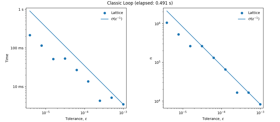

Classic-loop time and sample count versus tolerance.

Approach 2: Iteration log with resume

The solver first runs at the loosest tolerance and then resumes at progressively tighter tolerances. Because each resumed run starts from the previous state, the solver performs only the additional work needed for the new accuracy target.

After an initial or resumed run, get_iteration_log() returns a pandas DataFrame containing the stored iteration history. For QMC stopping criteria, the error surrogate is typically comb_bound_diff; for root-mean-square-error criteria, it may be rmse_estimate or rmse_tol. Resumed runs must use the same solver instance.

The panels below plot cumulative elapsed time and sample count against tolerance. Each point represents the work completed through that stopping point.

def collect_log_rows_resume(method_name, seed):
    """Resume through the tolerance sequence and return each stop row."""
    integ = qp.Keister(qp.Gaussian(qp.Lattice(3, seed=seed)))
    stopping_criterion = None
    data = None

    for eps in tol:  # loosest to tightest
        if stopping_criterion is None:
            stopping_criterion = qp.CubQMCLatticeG(
                integ, abs_tol=float(eps)
            )
            _, data = stopping_criterion.integrate()
        else:
            stopping_criterion.set_tolerance(abs_tol=float(eps))
            _, data = stopping_criterion.integrate(resume=data)

    result = stopping_criterion.get_iteration_log(
        formatted=False, view="stage_last"
    ).copy()
    result.insert(0, "method", method_name)
    result.insert(1, "abs_tol", np.asarray(tol)[: len(result)])
    columns = ["method", "abs_tol", "elapsed_time", "n_total"]
    return result[columns].sort_values(
        "abs_tol", ascending=False
    ).reset_index(drop=True)

approach2_tic = perf_counter()
iter_log = collect_log_rows_resume("Lattice", seed=7)
approach2_elapsed = perf_counter() - approach2_tic
print(f"Approach 2: elapsed={approach2_elapsed:.6f} s")

iter_log.head(9)

Approach 2: elapsed=0.210797 s

	method	absolute tolerance	cumulative time (s)	total samples
0	Lattice	0.001000	0.003221	8,192
1	Lattice	0.000500	0.005953	16,384
2	Lattice	0.000250	0.005953	16,384
3	Lattice	0.000125	0.016573	65,536
4	Lattice	0.000063	0.029973	131,072
5	Lattice	0.000031	0.056201	262,144
6	Lattice	0.000016	0.056201	262,144
7	Lattice	0.000008	0.109378	524,288
8	Lattice	0.000004	0.206681	1,048,576

plot_df = iter_log.copy()
plot_df[["abs_tol", "elapsed_time", "n_total"]] = plot_df[
    ["abs_tol", "elapsed_time", "n_total"]
].apply(pd.to_numeric, errors="coerce")
plot_df = plot_df.sort_values(["method", "abs_tol"])

def _positive_finite(values):
    values = np.asarray(values, dtype=float)
    return values[np.isfinite(values) & (values > 0)]

def draw_panel(axis, y_column, y_label):
    data = plot_df[plot_df["method"] == "Lattice"].sort_values(
        "abs_tol"
    )
    x = data["abs_tol"].to_numpy(dtype=float)
    y = data[y_column].to_numpy(dtype=float)
    reference = y[-1] * x[-1] / x

    axis.scatter(
        x, y, color="tab:blue", marker="o", s=50,
        label="Lattice", edgecolors="black",
    )
    axis.plot(
        x, reference, color="tab:blue", linewidth=2,
        label=r"$\mathcal{O}(\varepsilon^{-1})$",
    )

    values = _positive_finite(np.r_[y, reference])
    axis.set_xscale("log")
    axis.set_yscale("log")
    axis.set_xlim([x.min() * 0.8, x.max() * 1.2])
    axis.set_ylim([values.min() * 0.8, values.max() * 1.25])
    axis.set_xlabel("Tolerance, " + r"$\varepsilon$")
    axis.set_ylabel(y_label)
    axis.grid(True, which="major", alpha=0.25)
    axis.legend(frameon=False)
    axis.set_box_aspect(1)

fig2, ax2 = plt.subplots(
    1, 2, figsize=(12, 5.4), constrained_layout=True
)
fig2.suptitle(
    f"Iteration Log with Resume Workflow "
    f"(elapsed: {approach2_elapsed:.3f} s)"
)
draw_panel(ax2[0], "elapsed_time", "Time")
draw_panel(ax2[1], "n_total", "n")
ax2[0].yaxis.set_major_formatter(FuncFormatter(_time_fmt))
plt.show()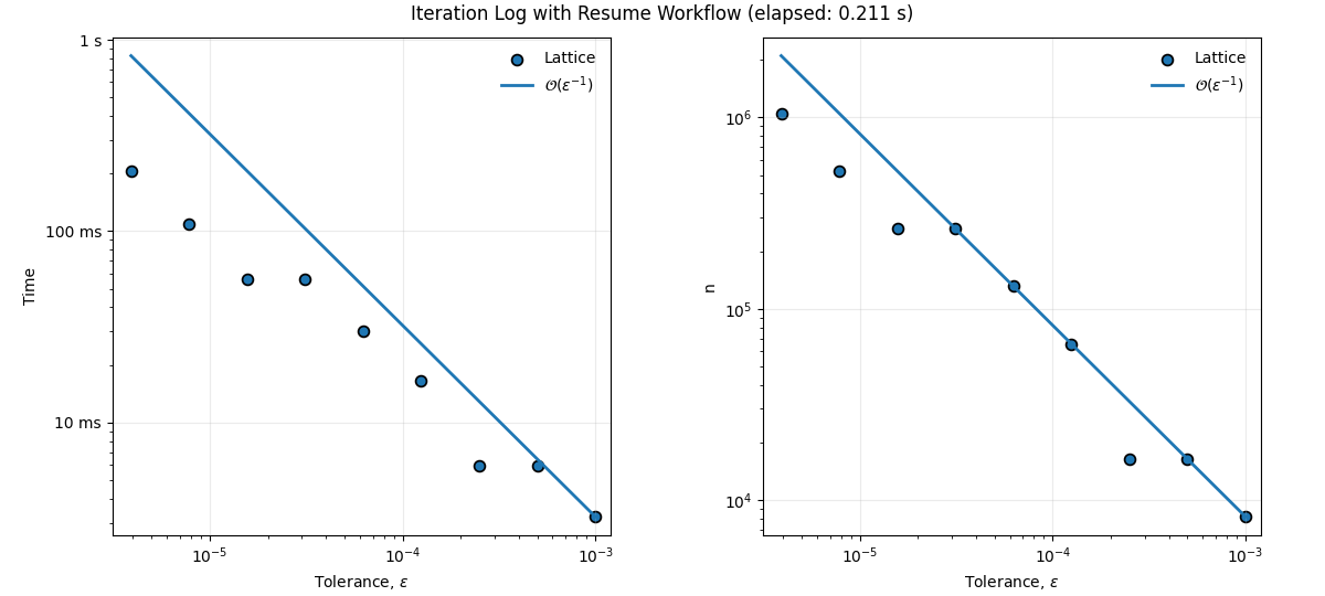

Iteration-log and resume time and sample count versus tolerance.

Although the two sets of plots look similar, the second workflow reuses prior work instead of starting fresh at every tolerance.

Repeated timing comparison

A single perf_counter() measurement is noisy, so the notebook also uses timeit.repeat() to run each workflow ten times.

import timeit

REPEAT = 10

def run_approach1_once():
    times, sample_counts = run_lattice_tolerance_curve(seed=7)
    return float(times.sum()), float(sample_counts[-1])

def run_approach2_once():
    log = collect_log_rows_resume("Lattice", seed=7)
    return (
        float(log["elapsed_time"].iloc[-1]),
        float(log["n_total"].iloc[-1]),
    )

def benchmark_callable(function, repeat=REPEAT):
    samples = np.asarray(
        timeit.repeat(function, number=1, repeat=repeat),
        dtype=float,
    )
    return pd.Series({
        "average": float(samples.mean()),
        "stdev": float(samples.std(ddof=1)),
        "min": float(samples.min()),
        "max": float(samples.max()),
        "repeat": int(repeat),
    })

benchmark_results = pd.DataFrame({
    "Classic Loop": benchmark_callable(run_approach1_once),
    "Iteration Log + Resume": benchmark_callable(run_approach2_once),
}).T
benchmark_results

workflow	average (s)	standard deviation (s)	minimum (s)	maximum (s)	repeats
Classic Loop	0.459063	0.006500	0.449794	0.469225	10
Iteration Log + Resume	0.212442	0.009557	0.202143	0.229744	10

Conclusion

For this multi-tolerance experiment, the iteration-log and resume workflow avoids repeatedly solving the same problem from scratch. It gives researchers access to the solver history and reuses completed work when the target tolerance is tightened.

The gain here applies to sequential tolerance exploration. If the final tight tolerance is already known, running directly at that tolerance remains the appropriate baseline.